
7.1. Motivating example: tracking location#
Suppose we let loose a cyborg corgi in a large park. We would like to know where it is at all time. For this purpose, it has an implanted location device that sends a signal to a tracking app.
Here is an example of the data we might have. The red dots are recorded locations at regular time intervals. The dotted line helps keep track of the time order of the recordings. (We will explain later how this dataset is generated.)
Show code cell source
ss = 4
os = 2
F = np.array([[1., 0., 1., 0.],[0., 1., 0., 1.],[0., 0., 1., 0.],[0., 0., 0., 1.]])
H = np.array([[1., 0., 0., 0.],[0., 1, 0., 0.]])
Q = 0.1 * np.diag(np.ones(ss))
R = 10 * np.diag(np.ones(os))
init_mu = np.array([0., 0., 1., 1.])
init_Sig = 1 * np.diag(np.ones(ss))
T = 50
x, y = mmids.lgSamplePath(ss, os, F, H, Q, R, init_mu, init_Sig, T)
plt.plot(y[0,:], y[1,:], marker='o', c='r', linestyle='dotted')
plt.xlim((np.min(y[0,:])-5, np.max(y[0,:])+5))
plt.ylim((np.min(y[1,:])-5, np.max(y[1,:])+5))
plt.show()
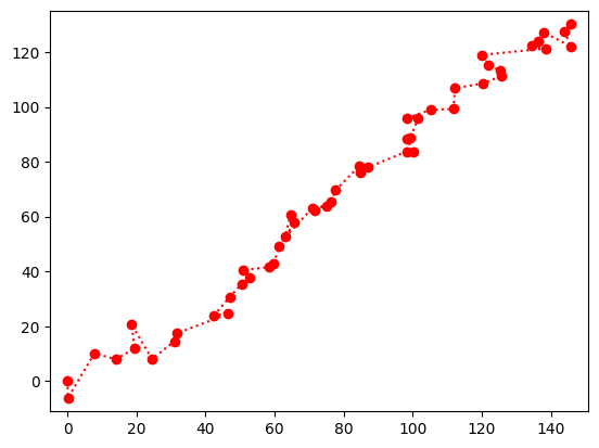
By convention, we start at \((0,0)\). Notice how squiggly the trajectory is. One issue might be that the times at which the location is recorded are too far between. But, in fact, there is another issue: the tracking device is inaccurate.
To get a better estimate of the true trajectory, it is natural to try to model the noise in the measurement as well as the dynamics itself. Probabilistic models are perfectly suited for this.
In this chapter, we will encounter of variety of such models and show how to take advantage of them to estimate unknown states (or parameters). In particular, conditional independence will play a key role.
We will come back to location tracking later in the chapter.