
\(\newcommand{\P}{\mathbb{P}}\) \(\newcommand{\E}{\mathbb{E}}\) \(\newcommand{\S}{\mathcal{S}}\) \(\newcommand{\var}{\mathrm{Var}}\) \(\newcommand{\bmu}{\boldsymbol{\mu}}\) \(\newcommand{\bSigma}{\boldsymbol{\Sigma}}\) \(\newcommand{\btheta}{\boldsymbol{\theta}}\) \(\newcommand{\bpi}{\boldsymbol{\pi}}\) \(\newcommand{\indep}{\perp\!\!\!\perp}\) \(\newcommand{\bp}{\mathbf{p}}\) \(\newcommand{\bx}{\mathbf{x}}\) \(\newcommand{\bX}{\mathbf{X}}\) \(\newcommand{\by}{\mathbf{y}}\) \(\newcommand{\bY}{\mathbf{Y}}\) \(\newcommand{\bz}{\mathbf{z}}\) \(\newcommand{\bZ}{\mathbf{Z}}\) \(\newcommand{\bw}{\mathbf{w}}\) \(\newcommand{\bW}{\mathbf{W}}\) \(\newcommand{\bv}{\mathbf{v}}\) \(\newcommand{\bV}{\mathbf{V}}\) \(\newcommand{\Z}{\mathcal{Z}}\) \(\newcommand{\bh}{\mathbf{h}}\) \(\newcommand{\bb}{\mathbf{b}}\) \(\newcommand{\bc}{\mathbf{c}}\) \(\newcommand{\cE}{\mathcal{E}}\) \(\newcommand{\cP}{\mathcal{P}}\)
7.5. Gibbs sampling with application to generating images#
In this section, we derive an important application of Markov chains known as Markov Chain Monte Carlo (MCMC). We specialize it to Gibbs sampling and apply it to the generation of handwritten digits using a Restricted Boltzmann Machine (RBM).
7.5.1. Markov chain Monte Carlo (MCMC)#
Suppose we are interested in generating samples from a target distribution \(\bpi = (\pi_i)_{i \in \S}\) over a set \(\S\). We have done this before. For instance, we generated samples from a mixture of Gaussians to test \(k\)-means clustering in different dimensions. There are many more applications. A canonical one is to estimate the mean of a function \(f\) under \(\bpi\): generate \(n\) independent samples \(Z_1,\ldots,Z_n\), all distributed according to \(\pi\), then compute
which is approximately \(\E[f(Z_1)]\) by the law of large numbers, provided \(n\) is sufficiently large. In particular, it plays an important role in Bayesian inference.
Sampling from simple distributions When \(\bpi\) is a standard distribution or \(\S\) is relatively small, this can be done efficiently by using a random number generator, as we have done previously.
NUMERICAL CORNER: Recall how this works. We first initialize the random number generator and use a seed for reproducibility.
seed = 535
rng = np.random.default_rng(seed)
To generate, say \(1000\), samples from a multivariate normal, say with mean \((0, 0)\) and covariance \(\begin{pmatrix}5 & 0\\0 & 1\end{pmatrix}\), we use numpy.random.Generator.multivariate_normal as follows.
mean = np.array([0., 0.])
cov = np.array([[5., 0.], [0., 1.]])
x, y = rng.multivariate_normal(mean, cov, 1000).T
Plotting the result we get:
Show code cell source
plt.scatter(x, y, marker='x')
plt.axis('equal')
plt.show()
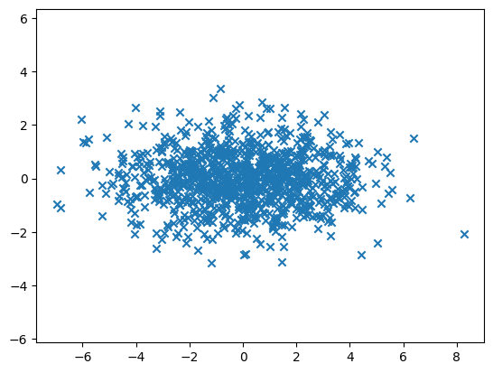
Computing the mean of each component we get:
print(np.mean(x))
-0.035322561120667575
print(np.mean(y))
-0.009499619370100139
This is somewhat close to the expected answer: \((0,0)\).
Using a larger number of samples, say \(10,000\), gives a better result.
x, y = rng.multivariate_normal(mean, cov, 10000).T
print(np.mean(x))
print(np.mean(y))
-0.0076273930440971215
-0.008874190869155479
\(\unlhd\)
Sampling from an arbitrary distribution on a finite set is also straightforward – as long as the set is not too big. This can be done using numpy.random.Generator.choice. Borrowing the example from the documentation, the following:
aa_milne_arr = ['pooh', 'rabbit', 'piglet', 'christopher']
rng.choice(aa_milne_arr, 5, p=[0.5, 0.1, 0.1, 0.3])
array(['pooh', 'pooh', 'piglet', 'christopher', 'piglet'], dtype='<U11')
generates \(5\) samples from the set \(\S = \{\tt{pooh}, \tt{rabbit}, \tt{piglet}, \tt{christopher}\}\) with respective probabilities \(0.5, 0.1, 0.1, 0.3\).
But this may not be practical when the state space \(\S\) is very large. As an example, later in this section, we will learn a “realistic” distribution of handwritten digits. We will do so using the MNIST dataset, which we have encountered previously.
We load it from PyTorch and turn the grayscale images (more precisely, each pixel is an integer between \(0\) and \(255\)) into a black-and-white images by rounding the pixels (after dividing by \(255\)).
Show code cell source
# Download and load the MNIST dataset
mnist = datasets.MNIST(root='./data',
                       train=True,
                       download=True,
                       transform=transforms.ToTensor())

# Convert the dataset to a PyTorch DataLoader
train_loader = torch.utils.data.DataLoader(mnist,
                                           batch_size=len(mnist),
                                           shuffle=False)

# Extract images and labels from the DataLoader
imgs, labels = next(iter(train_loader))
imgs = imgs.squeeze().numpy()
labels = labels.numpy()
imgs = np.round(imgs)
The first image is the following.
Show code cell source
plt.imshow(imgs[0], cmap=plt.cm.gray_r)
plt.show()
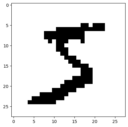
It is \(28 \times 28\), so the total number of pixels is \(784\).
nx_pixels, ny_pixels = imgs[0].shape
nx_pixels, ny_pixels
(28, 28)
n_pixels = nx_pixels * ny_pixels
n_pixels
784
To specify the a distribution over all possible black and white images of this size, we need in principle to assign a probability to a very large number of states. Our space here is \(\S = \{0,1\}^{784}\), imagining that \(0\) encodes white and \(1\) encodes black and that we have ordered the pixels in some arbitrary way. How big is this space?
Answer: \(2^{784}\).
Or in base \(10\), we compute \(\log_{10}(2^{784})\), which is:
784 * np.log(2) / np.log(10)
236.00751660056122
So a little more than \(10^{236}\).
This is much too large to naively plug into rng.choice!
So how to proceed? Instead we’ll use a Markov chain, as detailed next.
General setting The idea behind MCMC is simple. To generate samples from \(\bpi\), use a Markov chain \((X_t)_{t \geq 0}\) for which it is the stationary distribution. Indeed, we know from the Convergence to Equilibrium Theorem that if the chain is irreducible and aperiodic, then the distribution at time \(t\) is close to \(\bpi\) when \(t\) is large enough; and this holds for any initial dsitribution. Repeating this multiple times produces many independent, approximate samples from \(\bpi\).
The question is now:
How to construct a transition matrix \(P\) whose stationary distribution is given target distribution \(\bpi\)?
How to ensure that this Markov chain is relatively easy to simulate?
Regarding the first question, we have seen how to compute the stationary distribution of a transition matrix (provided it exists and is unique). How do we invert the process? Note one difficulty: many transition matrices can have the same stationary distribution. This is in fact a blessing, as it gives for designing a “good” Markov chain.
THINK-PAIR-SHARE: Construct two distinct transition matrices on \(2\) states whose stationary distribution is uniform. \(\ddagger\)
Regarding the second question, note that an obvious chain answering the first question is one that ignores the current state and chooses the next state according to \(\bpi\). We have already seen that this can be a problematic choice.
THINK-PAIR-SHARE: Show that this chain has the desired stationary distribution. \(\ddagger\)
Metropolis-Hastings We develop one standard technique that helps answer these two questions. It is known as the Metropolis-Hastings algorithm. It consists in two steps. We assume that \(\bpi > 0\), that is, \(\bpi_i > 0, \forall i \in \S\).
Proposal distribution: We first define a proposal chain, that is, a transition matrix \(Q\) on the space \(\S\). This chain does not need to have stationary distribution \(\bpi\). But it is typically a chain that is easy to simulate. A different way to think of this chain is that, for each state \(x \in \S\), we have a proposal distribution \(Q(x,\,\cdot\,)\) for the next state.
For instance, on the space of \(28 \times 28\) black-and-white images, we might pick a pixel uniformly at random and flip its value with probability \(1/2\).
MULTIPLE CHOICE: In the previous example, what is the stationary distribution?
a) All-white with probability \(1/2\), all-black with probability \(1/2\).
b) Uniform.
c) Too complex to compute.
d) What is a stationary distribution?
\(\ddagger\)
Hastings correction: At each step, we first pick a state according to \(Q\), given the current state. Then we accept or reject this move according to a specially defined probability that depends on \(Q\) as well as \(\bpi\). This is where the target distribution \(\bpi\) enters the picture, and the rejection probability is chosen to ensure that the new chain has the right stationary distribution, as we will see later. But first we define the full algorithm.
Formally, the algorithm goes as follows. Let \(x_0 \in \S\) be an arbitrary starting point and set \(X_0 := x_0\).
At each time \(t \geq 1\):
1- Pick a state \(Y\) according to the distribution \(Q(X_{t-1}, \,\cdot\,)\), that is, row \(X_{t-1}\) of \(Q\).
2- With probability
we set \(X_{t} := Y\) (i.e., we accept the move), and otherwise we set \(X_{t} := X_{t-1}\) (i.e., we reject the move).
YES or NO: Should we worry about the denominator \(\pi_{X_{t-1}} Q(X_{t-1}, Y)\) being \(0\)? \(\ddagger\)
We make three observations:
Taking a minimum with \(1\) ensures that acceptance probability is indeed between \(0\) and \(1\).
We only need to know \(\bpi\) up to a scaling factor since the chain depends only on the ratio \(\frac{\pi_{Y}}{\pi_{X_{t-1}}}\). The scaling factor cancels out. This turns out to be critical in many applications of MCMC. We will see an example in the next subsection.
If \(Q\) is symmetric, that is, \(Q(x,y) = Q(y,x)\) for all \(x, y \in \S\), then the ratio \(\frac{Q(Y, X_{t-1})}{Q(X_{t-1}, Y)}\) is just \(1\), leading to a simpler formula for the acceptance probability. In particular, in that case, moving to a state with a larger probability under \(\bpi\) is always accepted.
EXAMPLE: Suppose \(\S = \{1,\cdots, n\} = [n]\) for some positive integer \(n\) and \(\bpi\) is proportional to a Poisson distribution with mean \(\lambda > 0\). That is,
for some constant \(C\) chosen so that \(\sum_{i=1}^{n} \pi_i = 1\). Recall that we do not need to determine \(C\) as it is enough to know the target distribution up to a scaling factor by the previous remark.
To apply Metropolis-Hastings, we need a proposal chain. Consider the following choice. For each \(1 < i < n\), move to \(i+1\) or \(i-1\) with probability \(1/2\) each. For \(i=1\) (respectively \(i = n\)), move to \(2\) (respectively \(n-1\)) with probability \(1/2\), otherwise stay where you are. For instance, if \(n = 4\), then
which is indeed a stochastic matrix. It is also symmetric, so it does not enter into the acceptance probability by the previous remark.
To compute the acceptance probability, we only need to consider pairs of adjacent integers as they are the only one that have non-zero probability under \(Q\). Consider state \(1 < i < n\). Observe that
so a move to \(i+1\) happens with probability
where the \(1/2\) factor from the proposal distribution. Similarly, it can be checked (try it!) that a move to \(i-1\) occurs with probability
And we stay at \(i\) with probability \(1 - \frac{1}{2} \min\left\{1, \frac{\lambda}{i+1}\right\} - \frac{1}{2} \min\left\{1, \frac{i}{\lambda}\right\}\). (Why is this guaranteed to be a probability?)
A similar formula applies to \(i = 1, n\). (Try it!)
We are ready to apply Metropolis-Hastings.
def mh_transition_poisson(lmbd, n):
    P = np.zeros((n,n))
    for idx in range(n):
        i = idx + 1 # index starts at 0 rather than 1
        if (i > 1 and i < n):
            P[idx, idx+1] = (1/2) * np.min(np.array([1, lmbd/(i+1)]))
            P[idx, idx-1] = (1/2) * np.min(np.array([1, i/lmbd]))
            P[idx, idx] = 1 - P[idx, idx+1] - P[idx, idx-1]
        elif i == 1:
            P[idx, idx+1] = (1/2) * np.min(np.array([1, lmbd/(i+1)]))
            P[idx, idx] = 1 - P[idx, idx+1]
        elif i == n:
            P[idx, idx-1] = (1/2) * np.min(np.array([1, i/lmbd]))
            P[idx, idx] = 1 - P[idx, idx-1]
    return P
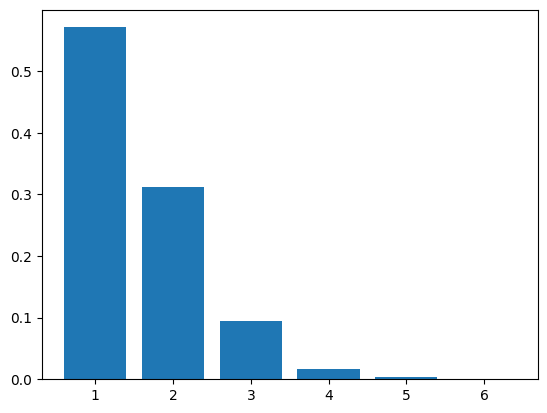
Take \(\lambda = 1\) and \(n = 6\). We get the following transition matrix.
lmbd = 1
n = 6
P = mh_transition_poisson(lmbd, n)
print(P)
[[0.75       0.25       0.         0.         0.         0.        ]
 [0.5        0.33333333 0.16666667 0.         0.         0.        ]
 [0.         0.5        0.375      0.125      0.         0.        ]
 [0.         0.         0.5        0.4        0.1        0.        ]
 [0.         0.         0.         0.5        0.41666667 0.08333333]
 [0.         0.         0.         0.         0.5        0.5       ]]
We use our simulator from a previous chapter. We start from the uniform distribution and take \(100\) steps.
mu = np.ones(n) / n
T = 100
X = mmids.SamplePath(mu, P, T)
Our sample is the final state of the trajectory.
X[T]
1.0
We repeat \(1000\) times and plot the frequencies.
N_samples = 1000 # number of repetitions

freq_z = np.zeros(n) # init of frequencies sampled
for i in range(N_samples):
    X = mmids.SamplePath(mu, P, T)
    freq_z[int(X[T])-1] += 1 # adjust for index starting at 0

freq_z = freq_z/N_samples
Show code cell source
plt.bar(range(1,n+1),freq_z)
plt.show()
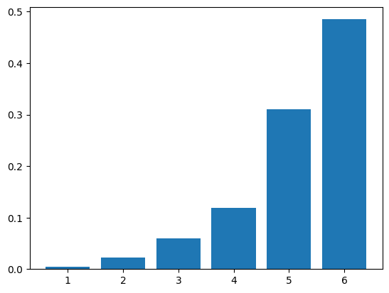
If we increase the parameter \(\lambda\) (which is not quite the mean; why?), we expect the sampled distribution to shift to the right. We must recompute the transition matrix first.
lmbd = 10
P = mh_transition_poisson(lmbd, n)
freq_z = np.zeros(n) # init of frequencies sampled
for i in range(N_samples):
    X = mmids.SamplePath(mu, P, T)
    freq_z[int(X[T])-1] += 1 # adjust for index starting at 0

freq_z = freq_z/N_samples
Show code cell source
plt.bar(range(1,n+1),freq_z)
plt.show()
TRY IT! Redo the simulations, but this time implement a general Metropolis-Hastings algorithm rather than specifying the transition matrix directly. That is, implement the algorithm for an arbitrary \(\bpi\) and \(Q\). Assume the state space is \([n]\). (Open in Colab)
\(\lhd\)
It remains to prove that \(\bpi\) is needed the stationary distribution of the Metropolis-Hastings algorithm. We restrict ourselves to the symmetric case, that is, \(Q(x,y) = Q(y,x)\) for all \(x,y\).
THEOREM (Correctness of Metropolis-Hastings) Consider the Metropolis-Hastings algorithm with target distribution \(\bpi\) over finite state space \(\S\) and symmetric proposal chain \(Q\). Assume further that \(\bpi\) is strictly positive and \(Q\) is irreducible over \(\S\). The resulting Markov chain is irreducible and reversible with respect to \(\bpi\). \(\sharp\)
Proof idea: It is just a matter of writing down the resulting transition matrix \(P\) and checking the detailed balance conditions. Because of the minimum in the acceptance probability, one has to consider two cases each time.
Proof: Let \(P\) denote the transition matrix of the resulting Markov chain. Our first task is to compute \(P\).
Let \(x, y \in \S\) be a pair of distinct states such that \(Q(x, y) = Q(y, x) = 0\). Then, from \(x\) (respectively \(y\)), the proposal chain never picks \(y\) (respectively \(x\)) as the possible next state. Hence \(P(x,y) = P(y, x) = 0\) in that case.
So let \(x, y \in \S\) be a pair of distinct states such that \(Q(x, y) = Q(y, x) > 0\). Applying the Hastings correction, we get that the overall probability of moving to \(y\) from current state \(x\) is
where we used the symmetry of \(Q\) and the notation \(a \land b = \min\{a,b\}\). Similarly,
Since \(P(x,y)\) is stricly positive exactly when \(Q(x,y)\) is strictly positive (for distinct \(x,y\)), the chain \(P\) has the same transition graph as the chain \(Q\). Hence, because \(Q\) is irreducible, so is \(P\).
It remains to check the detailed balance conditions. There are two cases. Without loss of generality, say \(\pi_x \leq \pi_y\). Then the previous formulas for \(P\) simplify to
Hence,
where we used the symmetry of \(Q\) to obtain the second equality. That establishes the reversibility of \(P\) and concludes the proof. \(\square\)
7.5.2. Gibbs sampling#
We have seen that one challenge of the Metropolis-Hastings approach is to choose a good proposal chain. Gibbs sampling is a canonical way of addressing this issue that has many applications. It applies in cases where the states are vectors, typically with a large number of coordinates, and where the target distribution has the kind of conditional independence properties we have encountered previously in this chapter.
General setting Here we will assume that \(\S = \Z^d\) where \(\Z\) is a finite set and \(d\) is the dimension. To emphasise that states are vectors, we will boldface letters, e.g., \(\bx = (x_i)_{i=1}^d\), \(\by = (y_i)_{i=1}^d\), etc., to denote them.
We will need the following special notation. For a vector \(\bx \in \Z^d\) and an index \(i \in [d]\), we write
for the vector \(\bx\) where the coordinate \(x_i\) is dropped.
If \(\pi\) is the target distribution, we let \(\pi_i(x_i|\bx_{-i})\) be the conditional probability that \(X_i = x_i\) given that \(\bX_{-i} = \bx_{-i}\) under the distribution \(\pi\), i.e., \(\bX = (X_1,\ldots,X_d) \sim \pi\). We assume that \(\pi_{\bx} > 0\) for all \(\bx \in \Z^d\). As a result, \(\pi_i(x_i|\bx_{-i}) > 0\) as well (Prove it!).
A basic version of the Gibbs sampler generates a sequence of vectors \(\bX_0, \bX_1, \ldots, \bX_t, \ldots\) in \(\Z^d\) as follows. We denote the coordinates of \(\bX_t\) by \((X_{t,1}, \ldots, X_{t,d})\). We denote the vector of all coordinates of \(\bX_t\) except \(i\) by \(\bX_{t,-i}\).
Pick \(\bX_0\) according to an arbitrary initial distribution \(\mu\) over \(\Z^d\).
At each time \(t \geq 1\):
1- Pick a coordinate \(i\) uniformly at random in \([d]\).
2- Update coordinate \(X_{t,i}\) according to \(\pi_i(\,\cdot\,|\bX_{t-1,-i})\) while leaving all other coordinates unchanged.
We will implement it in a special case in the next subsection. But first we argue that it has the desired stationary distribution.
It suffices to establish that the Gibbs sampler is a special case of the Metropolis-Hastings algorithm. For this, we must identify the appropriate proposal chain \(Q\).
We claim that the following choice works: for \(\bx \neq \by\),
The condition “\(\by_{-i} = \bx_{-i}\) for some \(i \in [d]\)” ensures that we only consider moves that affect a single coordinate \(i\). The factor \(1/d\) means that we pick that coordinate uniformly at random among all coordinates.
For each \(\bx\), we stay put with the remaining probability.
THINK-PAIR-SHARE: Write down explicitly the staying probability \(Q(\bx, \bx)\) and check it is indeed in \([0,1]\). \(\ddagger\)
In general, this \(Q\) is not symmetric. For \(\bx \neq \by\) with \(Q(\bx, \by) > 0\) where \(i\) is the non-matching coordinate, the acceptance probability is
where we used that \(\bx_{-i} = \by_{-i}\) in the second equality.
Recall the definition of the conditional probability as a ratio: \(\P[A|B] = \P[A\cap B]/\P[B]\). Applying that definition, both conditional probabilities \(\pi_i(x_i|\bx_{-i})\) and \(\pi_i(y_i|\bx_{-i})\) have the same denominator. Their respective numerators on the other hand are \(\pi_{\bx}\) and \(\pi_{\by}\). Hence,
In other words, the proposed move is always accepted! Therefore \(P = Q\), which is indeed the Gibbs sampler. It also establishes by Correctness of Metropolis-Hastings that \(P\) is reversible with respect to \(\pi\). It is also irreducible (Why?).
Here we picked a coordinate at random. It turns out that other choices are possible/ For example, one could update each coordinate in some deterministic order; or one could update blocks of coordinates at a time. Under some conditions, these schemes can still produce to an algorithm simulating the desired distribution. We will detail this here, but our implementation below does use a block scheme.
An example: restricted Boltzmann machines (RBM) We implement the Gibbs sampler on a specific probabilistic model, a so-called restricted Boltzmann machine (RBM), and apply it to the generation of random images from a “realistic” distribution. For more on Boltzmann machines, including their restricted and deep versions, see here. We will not describe them in great details here, but only use them as an example of a complex distribution.
Probabilistic model: An RBM has \(m\) visible units (i.e., observed variables) and \(n\) hidden units (i.e., hidden variables). It is represented by a complete bipartite graph between the two.
Figure: An RBM (Source)

\(\bowtie\)
Visible unit \(i\) is associated a variable \(v_i\) and hidden unit \(j\) is associated a variable \(h_j\). We define the corresponding vectors \(\bv = (v_1,\ldots,v_m)\) and \(\bh = (h_1,\ldots,h_n)\). For our purposes, it will suffice to assume that \(\bv \in \{0,1\}^m\) and \(\bh \in \{0,1\}^n\). These are referred to as binary units.
The probabilistic model has a number of parameters. Each visible unit \(i\) has an offset \(b_i \in \mathbb{R}\) and each hidden unit \(j\) has an offset \(c_j \in \mathbb{R}\). We write \(\bb = (b_1,\ldots,b_m)\) and \(\bc = (c_1,\ldots,c_n)\) for the offset vectors. For each pair \((i,j)\) of visible and hidden units (or, put differently, for each edge in the complete bipartite graph), there is a weight \(w_{i,j} \in \mathbb{R}\). We write \(W = (w_{i,j})_{i,j=1}^{m,n}\) for the weight matrix.
To define the probability distribution, we need the so-called energy (as you may have guessed, this terminology comes from related models in physics): for \(\bv \in \{0,1\}^m\) and \(\bh \in \{0,1\}^n\),
The joint distribution of \(\bv\) and \(\bh\) is
where \(Z\), the partition function (a function of \(W,\bb,\bc\)), ensures that \(\pi\) indeed sums to \(1\).
We will be interested in sampling from the marginal over visible units, that is,
When \(m\) and/or \(n\) are large, computing \(\rho\) or \(\pi\) explicitly – or even numerically – is impractical.
We develop the Gibbs sampler for this model next.
Gibbs sampling: We sample from the joint distribution \(\pi\) and observe only \(\bv\).
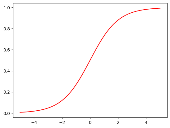
We need to compute the conditional probabilities given every other variable. The sigmoid function, which we have encountered previously,
will once again make an appearance.
def sigmoid(x):
    return 1/(1 + np.exp(-x))
Show code cell source
grid = np.linspace(-5, 5, 100)
plt.plot(grid,sigmoid(grid),'r')
plt.show()
Fix a visible unit \(i \in [m]\). For a pair \((\bv, \bh)\), we denote by \((\bv_{[i]}, \bh)\) the same pair where coordinate \(i\) of \(\bv\) is flipped. Given every other variable, i.e., \((\bv_{-i},\bh)\), and using a superscript \(\text{v}\) to indicate the probability of a visible unit, the conditional probability of \(v_i\) is
In this last ratio, the partition functions (the \(Z\)’s) cancel out. Moreover, all the terms in the exponentials not depending on the \(i\)-th visible unit actually factor out and cancel out as well – they are identical in all three exponentials. Similarly, the terms in the exponentials depending only on \(\bh\) also factor out and cancel out.
What we are left with is:
where we used the fact that flipping \(v_i \in \{0,1\}\) is the same as setting it to \(1 - v_i\), a transformation which indeed sends \(0\) to \(1\) and \(1\) to \(0\).
This expression does not depend on \(\bv_{-i}\). In other words, the \(i\)-th visible unit is conditionally independent of all other visible units given the hidden units.
We simplify the expression
In particular, the conditional mean of the \(i\)-th visible unit given everything else is
Similarly for the conditional of the \(j\)-th hidden unit given everything else, we have
The conditional mean given everything else is
And the \(j\)-th hidden unit is conditionally independent of all other hidden units given the visible units.
NUMERICAL CORNER: We implement the Gibbs sampler for an RBM. Rather than updating the units at random, we use a block approach. Specifically, we update all hidden units independently, given the visible units; then we update all visible units independently, given the hidden units. In each case, this is warranted by the conditional independence structure revealed above.
We first implement the conditional means using the formulas previously derived.
def rbm_mean_hidden(v, W, c):
    return sigmoid(W @ v + c)
def rbm_mean_visible(h, W, b):
    return sigmoid(W.T @ h + b)
We next implement one step of the sampler, which consists in updating all hidden units, followed by updating all visible units.
def rbm_gibbs_update(v, W, b, c):
    p_hidden = rbm_mean_hidden(v, W, c)
    h = rng.binomial(1, p_hidden, p_hidden.shape)
    p_visible = rbm_mean_visible(h, W, b)
    v = rng.binomial(1, p_visible, p_visible.shape)
    return v
Finally, we repeat these steps k times. We only return the visible units v.
def rbm_gibbs_sampling(k, v_0, W, b, c):
    counter = 0
    v = v_0
    while counter < k:
        v = rbm_gibbs_update(v, W, b, c)
        counter += 1
    return v
Here v_0 is the initial visible unit states. We do not need to initialize the hidden ones as this is done automatically in the first update step. In the next subsection, we will take the initial distribution of \(\bv\) to be independent Bernoullis with success probability \(1/2\).
\(\unlhd\)
7.5.3. Sampling handwritten digits with an RBM#
We apply our Gibbs sampler to generating images. As mentioned previously, we use the MNIST dataset to learn a “realistic” distribution of handwritten digit images. Here the images are encoded by the visible units of an RBM. Then we sample from this model.
Trainging the model We first need to train the model on the data. We will not show how this is done here, but instead use sklearn.neural_network.BernoulliRBM. (Some details of how this training is done is provided here.)
from sklearn.neural_network import BernoulliRBM
rbm = BernoulliRBM(random_state=seed, verbose=0)
To simplify the analysis and speed up the training, we only keep digits \(0\), \(1\) and \(5\).
# Filter out images with labels 0, 1, or 5
mask = (labels == 0) | (labels == 1) | (labels == 5)
imgs = imgs[mask]
labels = labels[mask]
We flatten the images (which have already been “rounded” to black-and-white; see the first subsection).
X = imgs.reshape(len(imgs), -1)
We now fit the model. Choosing the hyperparameters of the training algorithm is tricky. The following seem to work reasonably well. (For a more systematic approach to tuning hyperparameters, see here.)
rbm.n_components = 100
rbm.learning_rate = 0.02
rbm.batch_size = 50
rbm.n_iter = 20
rbm.fit(X)
BernoulliRBM(batch_size=50, learning_rate=0.02, n_components=100, n_iter=20,
             random_state=535)
In a Jupyter environment, please rerun this cell to show the HTML representation or trust the notebook. On GitHub, the HTML representation is unable to render, please try loading this page with nbviewer.org.
BernoulliRBM(batch_size=50, learning_rate=0.02, n_components=100, n_iter=20,
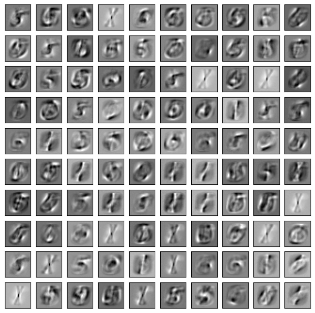
random_state=535)We plot the learned weight matrix using a script adapted from here. Each image shows the weights associated to all visible units by one hidden unit.
def plot_imgs(z, n_imgs, nx_pixels, ny_pixels):
    nx_imgs = np.floor(np.sqrt(n_imgs))
    ny_imgs = np.ceil(np.sqrt(n_imgs))
    plt.figure(figsize=(8, 8))
    for i, comp in enumerate(z):
        plt.subplot(int(nx_imgs), int(ny_imgs), i + 1)
        plt.imshow(comp.reshape((nx_pixels, ny_pixels)),
                   cmap=plt.cm.gray_r)
        plt.xticks([])
        plt.yticks([])
    plt.show()
Show code cell source
plot_imgs(rbm.components_, rbm.n_components,
          nx_pixels, ny_pixels)
Back to Gibbs sampling We are ready to sample from the trained RBM. We extract the learned parameters from rbm.
W = rbm.components_
W.shape
(100, 784)
b = rbm.intercept_visible_
b.shape
(784,)
c = rbm.intercept_hidden_
c.shape
(100,)
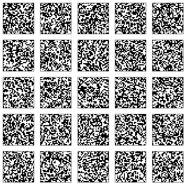
To generate \(25\) samples, we first generate \(25\) independent initial states. We stack them into a matrix, where each row is a different flattened random noise image.
n_samples = 25 # number of samples
z = rng.binomial(1, 0.5, (n_samples, n_pixels))
Show code cell source
plot_imgs(z, n_samples, nx_pixels, ny_pixels)
To process all samples simultaneously, we make a small change to the code. We numpy.reshape
to make the offsets into column vectors, which are then automatically added to all columns of the resulting weighted sum.
(This is known as broadcasting.)
def rbm_mean_hidden(v, W, c):
    return sigmoid(W @ v + c.reshape(len(c),1))
def rbm_mean_visible(h, W, b):
    return sigmoid(W.T @ h + b.reshape(len(b),1))
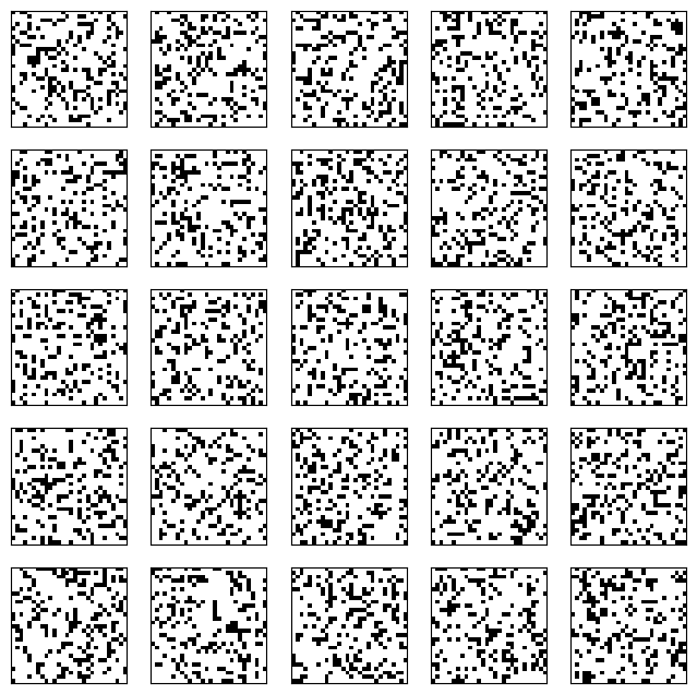
We are now ready to run our Gibbs sampler. The outcome depends on the number of steps we take. For instance, after one step, the result is still very noisy – although note that the fraction of white pixels is already more realistic!
v_0 = z.T
gen_v = rbm_gibbs_sampling(1, v_0, W, b, c)
Show code cell source
plot_imgs(gen_v.T, n_samples, nx_pixels, ny_pixels)
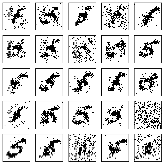
After \(10\) steps, we already see shadows of digits appearing.
v_0 = z.T
gen_v = rbm_gibbs_sampling(10, v_0, W, b, c)
Show code cell source
plot_imgs(gen_v.T, n_samples, nx_pixels, ny_pixels)
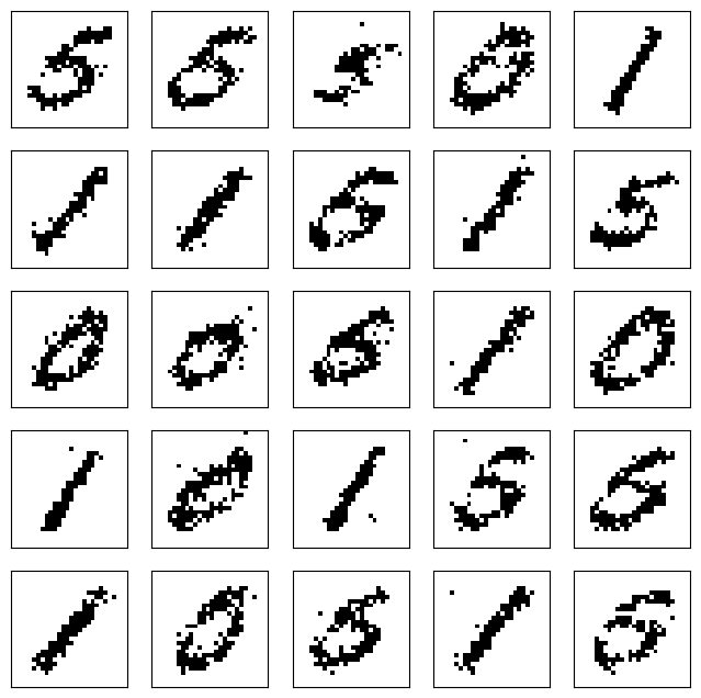
After \(100\) steps, the outcome is quite realistic.
v_0 = z.T
gen_v = rbm_gibbs_sampling(100, v_0, W, b, c)
Show code cell source
plot_imgs(gen_v.T, n_samples, nx_pixels, ny_pixels)
RBMs can be stacked into deep probabilistic models, similarly to what we encountered with neural networks.