1.1. Motivating example: identifying penguin species

Imagine that you are an evolutionary biologist studying penguins. You have collected measurements on a large number of individual specimens. Your goal is to identify different species within this collection based on those measurements.

Figure: An Adelie penguin (Source)

\(\bowtie\)

Here is a penguin dataset collected and made available by Dr. Kristen Gorman and the Palmer Station, Antarctica LTER. We will upload the data in the form of a data table (similar to a spreadsheet) called DataFrame in pandas, where the columns are different measurements (or features) and the rows are different samples. Below, we load the data using pandas.read_csv and show the first \(5\) lines of the dataset (see DataFrame.head). This dataset is a simplified version (i.e., with some columns removed) of the full dataset, maintained by Allison Horst at this GitHub page.

import pandas as pd

df = pd.read_csv('penguins-measurements.csv')
df.head()

	bill_length_mm	bill_depth_mm	flipper_length_mm	body_mass_g
0	39.1	18.7	181.0	3750.0
1	39.5	17.4	186.0	3800.0
2	40.3	18.0	195.0	3250.0
3	NaN	NaN	NaN	NaN
4	36.7	19.3	193.0	3450.0

Observe that this dataset has missing values (i.e., the entries NaN above). A common way to deal with this issue is to remove all rows with missing values. This can be done using pandas.DataFrame.dropna. This kind of pre-processing is fundamental in data science, but we will not discuss it much in this course.

df = df.dropna()
df.head()

	bill_length_mm	bill_depth_mm	flipper_length_mm	body_mass_g
0	39.1	18.7	181.0	3750.0
1	39.5	17.4	186.0	3800.0
2	40.3	18.0	195.0	3250.0
4	36.7	19.3	193.0	3450.0
5	39.3	20.6	190.0	3650.0

There are \(342\) samples, as can be seen by using pandas.DataFrame.shape which gives the dimensions of the DataFrame as a tuple.

df.shape

(342, 4)

Here is a summary of the data (see pandas.DataFrame.describe).

df.describe()

	bill_length_mm	bill_depth_mm	flipper_length_mm	body_mass_g
count	342.000000	342.000000	342.000000	342.000000
mean	43.921930	17.151170	200.915205	4201.754386
std	5.459584	1.974793	14.061714	801.954536
min	32.100000	13.100000	172.000000	2700.000000
25%	39.225000	15.600000	190.000000	3550.000000
50%	44.450000	17.300000	197.000000	4050.000000
75%	48.500000	18.700000	213.000000	4750.000000
max	59.600000	21.500000	231.000000	6300.000000

Let’s first extract the columns into a Numpy array using pandas.DataFrame.to_numpy().

X = df.to_numpy()
print(X)

[[  39.1   18.7  181.  3750. ]
 [  39.5   17.4  186.  3800. ]
 [  40.3   18.   195.  3250. ]
 ...
 [  50.4   15.7  222.  5750. ]
 [  45.2   14.8  212.  5200. ]
 [  49.9   16.1  213.  5400. ]]

We visualize two measurements in the data, the bill depth and flipper length. (The original dataset used the more precise term culmen depth.) Below, each point is a sample. This is called a scatter plot. We use matplotlib.pyplot for most of our plotting needs in this book, with a few exceptions (see below). Specifically, here we use the function matplotlib.pyplot.scatter.

import matplotlib.pyplot as plt

plt.scatter(X[:,1], X[:,2], s=10)
plt.xlabel('bill_depth_mm')
plt.ylabel('flipper_length_mm')
plt.show()

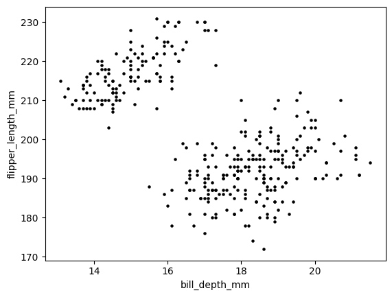
We observe what appears to be two fairly well-defined clusters of samples on the top left and bottom right respectively. What is a cluster? Intuitively, it is a group of samples that are close to each other, but far from every other sample. In this case, it may be an indication that these samples come from a separate species.

Now let’s look at the full dataset. Visualizing the full \(4\)-dimensional data is not straightforward. One way to do this is to consider all pairwise scatter plots. We use the function seaborn.pairplot from the library Seaborn.

Show code cell source Hide code cell source

import seaborn as sns

Show code cell source Hide code cell source

sns.pairplot(df, height=1.5)
plt.show()

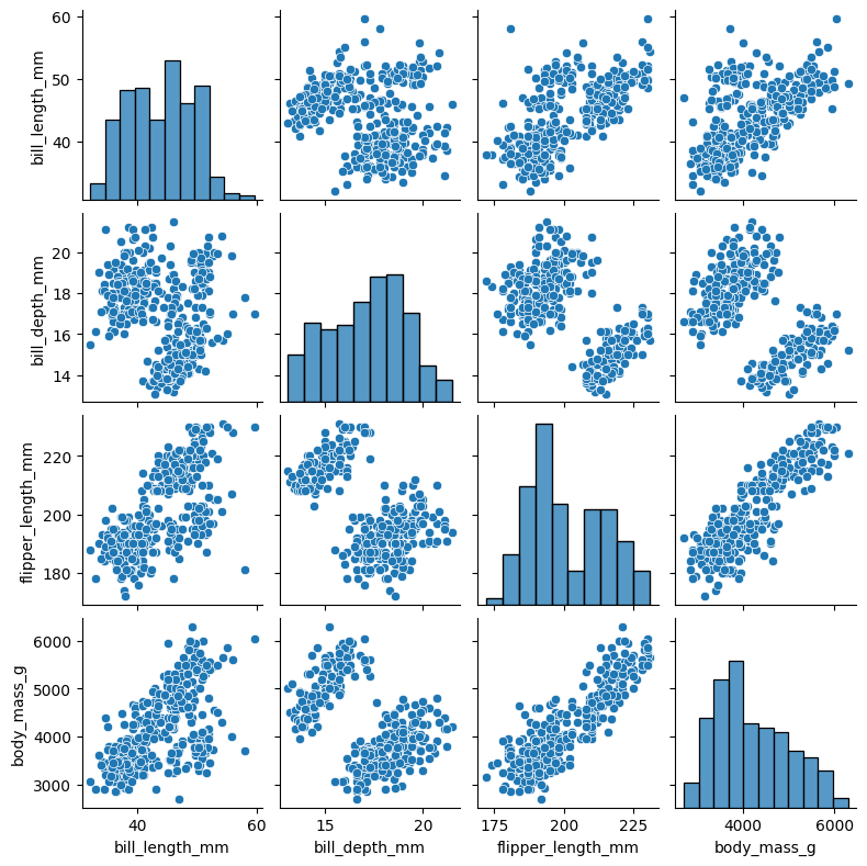
NUMERIC ANSWER: How many species of penguins do you think there are in this dataset? \(\ddagger\)

What would be useful is a method that automatically identifies clusters whatever the dimension of the data. In this chapter, we will discuss a standard way to do this: \(k\)-means clustering. We will come back to the penguins dataset later in the chapter.

But first we need to review some basic concepts about vectors and distances in order to formulate clustering as an appropriate optimization problem, a perspective that will be recurring throughout.

LEARNING BY CHATTING Ask your favorite AI chatbot for alternative ways to deal with missing values in a dataset. Implement one of these alternatives on the penguins dataset (ask the chatbot for the code). (Open in Colab)