Background: review of vector spaces and matrix inverses

$\newcommand{\bmu}{\boldsymbol{\mu}}$ $\newcommand{\bSigma}{\boldsymbol{\Sigma}}$ $\newcommand{\bfbeta}{\boldsymbol{\beta}}$ $\newcommand{\bflambda}{\boldsymbol{\lambda}}$ $\newcommand{\bgamma}{\boldsymbol{\gamma}}$ $\newcommand{\bsigma}{{\boldsymbol{\sigma}}}$ $\newcommand{\bpi}{\boldsymbol{\pi}}$ $\newcommand{\btheta}{{\boldsymbol{\theta}}}$ $\newcommand{\bphi}{\boldsymbol{\phi}}$ $\newcommand{\balpha}{\boldsymbol{\alpha}}$ $\newcommand{\blambda}{\boldsymbol{\lambda}}$ $\renewcommand{\P}{\mathbb{P}}$ $\newcommand{\E}{\mathbb{E}}$ $\newcommand{\indep}{\perp\!\!\!\perp} \newcommand{\bx}{\mathbf{x}}$ $\newcommand{\bp}{\mathbf{p}}$ $\renewcommand{\bx}{\mathbf{x}}$ $\newcommand{\bX}{\mathbf{X}}$ $\newcommand{\by}{\mathbf{y}}$ $\newcommand{\bY}{\mathbf{Y}}$ $\newcommand{\bz}{\mathbf{z}}$ $\newcommand{\bZ}{\mathbf{Z}}$ $\newcommand{\bw}{\mathbf{w}}$ $\newcommand{\bW}{\mathbf{W}}$ $\newcommand{\bv}{\mathbf{v}}$ $\newcommand{\bV}{\mathbf{V}}$ $\newcommand{\bfg}{\mathbf{g}}$ $\newcommand{\bfh}{\mathbf{h}}$ $\newcommand{\horz}{\rule[.5ex]{2.5ex}{0.5pt}}$ $\renewcommand{\S}{\mathcal{S}}$ $\newcommand{\X}{\mathcal{X}}$ $\newcommand{\var}{\mathrm{Var}}$ $\newcommand{\pa}{\mathrm{pa}}$ $\newcommand{\Z}{\mathcal{Z}}$ $\newcommand{\bh}{\mathbf{h}}$ $\newcommand{\bb}{\mathbf{b}}$ $\newcommand{\bc}{\mathbf{c}}$ $\newcommand{\cE}{\mathcal{E}}$ $\newcommand{\cP}{\mathcal{P}}$ $\newcommand{\bbeta}{\boldsymbol{\beta}}$ $\newcommand{\bLambda}{\boldsymbol{\Lambda}}$ $\newcommand{\cov}{\mathrm{Cov}}$ $\newcommand{\bfk}{\mathbf{k}}$ $\newcommand{\idx}[1]{}$ $\newcommand{\xdi}{}$

2.2. Background: review of vector spaces and matrix inverses#

In this section, we introduce some basic linear algebra concepts that will be needed throughout this chapter and later on.

2.2.1. Subspaces#

We work over the vector space $V = \mathbb{R}^n$. We begin with the concept of a linear subspace.

DEFINITION (Linear Subspace) $\idx{linear subspace}\xdi$ A linear subspace of $\mathbb{R}^n$ is a subset $U \subseteq \mathbb{R}^n$ that is closed under vector addition and scalar multiplication. That is, for all $\mathbf{u}_1, \mathbf{u}_2 \in U$ and $\alpha \in \mathbb{R}$, it holds that

\[ \mathbf{u}_1 + \mathbf{u}_2 \in U \quad \text{and} \quad \alpha \,\mathbf{u}_1 \in U. \]

It follows from this condition that $\mathbf{0} \in U$. $\natural$

Alternatively, we can check these conditions by proving that (1) $\mathbf{0} \in U$ and (2) $\mathbf{u}_1, \mathbf{u}_2 \in U$ and $\alpha \in \mathbb{R}$ imply that $\alpha \mathbf{u}_1 + \mathbf{u}_2 \in U$. Indeed, taking $\alpha = 1$ gives the first condition above, while choosing $\mathbf{u}_2 = \mathbf{0}$ gives the second one.

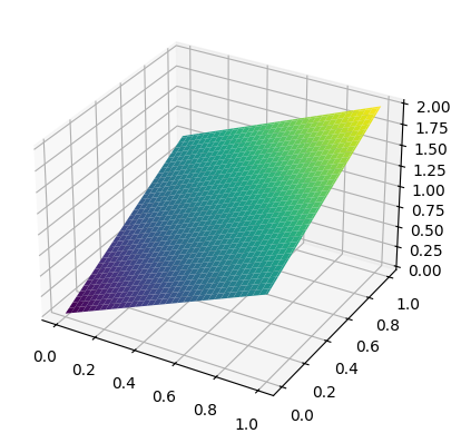
NUMERICAL CORNER: The plane $P$ made of all points $(x,y,z) \in \mathbb{R}^3$ that satisfy $z = x+y$ is a linear subspace. Indeed, $0 = 0 + 0$ so $(0,0,0) \in P$. And, for any $\mathbf{u}_1 = (x_1, y_1, z_1)$ and $\mathbf{u}_2 = (x_2, y_2, z_2)$ such that $z_1 = x_1 + y_1$ and $z_2 = x_2 + y_2$ and for any $\alpha \in \mathbb{R}$, we have

\[ \alpha z_1 + z_2 = \alpha (x_1 + y_1) + (x_2 + y_2) = (\alpha x_1 + x_2) + (\alpha y_1 + y_2). \]

That is, $\alpha \mathbf{u}_1 + \mathbf{u}_2$ satisfies the condition defining $P$ and therefore is itself in $P$. Note also that $P$ passes through the origin.

In this example, the linear subspace $P$ can be described alternatively as the collection of every vector of the form $(x, y, x+y)$.

We use plot_surface to plot it over a grid of points created using numpy.meshgrid.

x = np.linspace(0,1,num=101)
y = np.linspace(0,1,num=101)
X, Y = np.meshgrid(x, y)
print(X)

[[0.   0.01 0.02 ... 0.98 0.99 1.  ]
 [0.   0.01 0.02 ... 0.98 0.99 1.  ]
 [0.   0.01 0.02 ... 0.98 0.99 1.  ]
 ...
 [0.   0.01 0.02 ... 0.98 0.99 1.  ]
 [0.   0.01 0.02 ... 0.98 0.99 1.  ]
 [0.   0.01 0.02 ... 0.98 0.99 1.  ]]

print(Y)

[[0.   0.   0.   ... 0.   0.   0.  ]
 [0.01 0.01 0.01 ... 0.01 0.01 0.01]
 [0.02 0.02 0.02 ... 0.02 0.02 0.02]
 ...
 [0.98 0.98 0.98 ... 0.98 0.98 0.98]
 [0.99 0.99 0.99 ... 0.99 0.99 0.99]
 [1.   1.   1.   ... 1.   1.   1.  ]]

Z = X + Y
print(Z)

[[0.   0.01 0.02 ... 0.98 0.99 1.  ]
 [0.01 0.02 0.03 ... 0.99 1.   1.01]
 [0.02 0.03 0.04 ... 1.   1.01 1.02]
 ...
 [0.98 0.99 1.   ... 1.96 1.97 1.98]
 [0.99 1.   1.01 ... 1.97 1.98 1.99]
 [1.   1.01 1.02 ... 1.98 1.99 2.  ]]

fig = plt.figure()
ax = fig.add_subplot(111, projection='3d')
ax.plot_surface(X, Y, Z, cmap='viridis')
plt.show()

../../_images/4de151ba715b07481dc10ccb03213f013fc5adab2dddab2ce268b2afdfc9a5c8.png

$\unlhd$

Here is a key example of a linear subspace.

DEFINITION (Span) $\idx{span}\xdi$ Let $\mathbf{w}_1, \ldots, \mathbf{w}_m \in \mathbb{R}^n$. The span of $\{\mathbf{w}_1, \ldots, \mathbf{w}_m\}$, denoted $\mathrm{span}(\mathbf{w}_1, \ldots, \mathbf{w}_m)$, is the set of all linear combinations of the $\mathbf{w}_j$’s. That is,

\[ \mathrm{span}(\mathbf{w}_1, \ldots, \mathbf{w}_m) = \left\{ \sum_{j=1}^m \alpha_j \mathbf{w}_j\,:\, \alpha_1,\ldots, \alpha_m \in \mathbb{R} \right\}. \]

By convention, we declare that the span of the empty list is $\{\mathbf{0}\}$. $\natural$

EXAMPLE: (continued) In the example above, we noted that the plane $P$ is the collection of every vector of the form $(x, y, x+y)$. These can be written as $x \,\mathbf{w}_1 + y \,\mathbf{w}_2$ where $\mathbf{w}_1 = (1,0,1)$ and $\mathbf{w}_2 = (0,1,1)$, and vice versa. Hence $P = \mathrm{span}(\mathbf{w}_1,\mathbf{w}_2)$. $\lhd$

We check next that a span is indeed a linear subspace.

LEMMA Let $W=\mathrm{span}(\mathbf{w}_1, \ldots, \mathbf{w}_m)$. Then $W$ is a linear subspace. $\flat$

We say that $\mathbf{w}_1, \ldots, \mathbf{w}_m$ span $W$.

Proof: First, $\mathbf{0} = \sum_{j=1}^m 0\mathbf{w}_j \in W$. Second, let $\mathbf{u}_1, \mathbf{u}_2 \in W$ and $\alpha \in \mathbb{R}$. For $i=1,2$, because $\mathbf{u}_i$ is in the span of the $\mathbf{w}_j$’s, we can write

\[ \mathbf{u}_i = \sum_{j=1}^m \beta_{ij} \mathbf{w}_j \]

for some $\beta_{ij} \in \mathbb{R}$ for $j=1,\ldots,m$.

Therefore

\[ \alpha \mathbf{u}_1 + \mathbf{u}_2 = \alpha \sum_{j=1}^m \beta_{1j} \mathbf{w}_j + \sum_{j=1}^m \beta_{2j} \mathbf{w}_j = \sum_{j=1}^m (\alpha \beta_{1j} + \beta_{2j}) \mathbf{w}_j. \]

So $\alpha \,\mathbf{u}_1 + \mathbf{u}_2 \in W$.$\square$

CHAT & LEARN Consider the following problem:

Prove that if $\{\mathbf{v}_1,\ldots,\mathbf{v}_n\}$ spans $U$, then so does the list

\[ \{\mathbf{v}_1-\mathbf{v}_2, \mathbf{v}_2-\mathbf{v}_3,\ldots,\mathbf{v}_{n-1}-\mathbf{v}_n,\mathbf{v}_n\}, \]

obtained by subtracting from each vector (except the last one) the following vector.

A popular AI chatbot (which shall remain nameless) provided the following solution:

Suppose that $U = \text{span}(\mathbf{v}_1, \ldots, \mathbf{v}_n)$. Then for any vector $\mathbf{v} \in U$, there exist scalars $a_1, \ldots, a_n \in \mathbb{R}$ such that:

\[ \mathbf{v} = a_1\mathbf{v}_1 + a_2\mathbf{v}_2 + \ldots + a_n\mathbf{v}_n \]

Now let’s express each vector in the new list in terms of the given vectors:

$\mathbf{v}_1-\mathbf{v}_2 = a_1(\mathbf{v}_1-\mathbf{v}_2)$

$\mathbf{v}_2-\mathbf{v}_3 = (a_1 + a_2)(\mathbf{v}_2-\mathbf{v}_3)$

$\mathbf{v}_3-\mathbf{v}_4 = (a_1 + a_2 + a_3)(\mathbf{v}_3-\mathbf{v}_4)$

$\ldots$

$\mathbf{v}_{n-1} - \mathbf{v}_n = (a_1 + a_2 + \ldots + a_{n-1})(\mathbf{v}_{n-1}-\mathbf{v}_n)$

Adding up all these expressions, we get:

\[ \mathbf{v} = a_1(\mathbf{v}_1-\mathbf{v}_2) + (a_1 + a_2)(\mathbf{v}_2-\mathbf{v}_3) + \ldots + (a_1 + a_2 + \ldots + a_{n-1})(\mathbf{v}_{n-1}-\mathbf{v}_n) + a_n\mathbf{v}_n \]

This shows that $\mathbf{v}$ can be expressed as a linear combination of the vectors in the new list, which means that the new list also spans $U$. Therefore, the list ${\mathbf{v}_1-\mathbf{v}_2, \mathbf{v}_2-\mathbf{v}_3, \ldots, \mathbf{v}_{n-1}-\mathbf{v}_n, \mathbf{v}_n}$ spans $U$, completing the proof.

Explain everything that is wrong with this answer and provide a correct alternative proof. $\ddagger$

In matrix form, we talk about the column space of a (not necessarily square) matrix.

DEFINITION (Column Space) $\idx{column space}\xdi$ Let $A \in \mathbb{R}^{n\times m}$ be an $n\times m$ matrix with columns $\mathbf{a}_1,\ldots, \mathbf{a}_m \in \mathbb{R}^n$. The column space of $A$, denoted $\mathrm{col}(A)$, is the span of the columns of $A$, that is, $\mathrm{col}(A) = \mathrm{span}(\mathbf{a}_1,\ldots, \mathbf{a}_m)$. $\natural$

When thinking of $A$ as a linear map, that is, the vector-valued function $f(\mathbf{x}) = A \mathbf{x}$ mapping inputs in $\mathbb{R}^{m}$ to outputs in $\mathbb{R}^n$, the column space is referred to as the range or image.

We will need another important linear subspace defined in terms of a matrix.

DEFINITION (Null Space) $\idx{null space}\xdi$ Let $B \in \mathbb{R}^{n \times m}$. The null space of $B$ is the linear subspace

\[ \mathrm{null}(B) = \left\{\mathbf{x} \in \mathbb{R}^m\,:\, B\mathbf{x} = \mathbf{0}\right\}. \]

$\natural$

It can be shown that the null space is a linear subspace. We give a simple example next.

EXAMPLE: (continued) Going back to the linear subspace $P = \{(x,y,z)^T \in \mathbb{R}^3 : z = x + y\}$, the condition in the definition can be re-written as $x + y - z = 0$. Hence $P = \mathrm{null}(B)$ for the single-row matrix $B = \begin{pmatrix} 1 & 1 & - 1\end{pmatrix}$. $\lhd$

2.2.2. Linear independence and bases#

It is often desirable to avoid redundancy in the description of a linear subspace.

We start with an example.

EXAMPLE: Consider the linear subspace $\mathrm{span}(\mathbf{w}_1,\mathbf{w}_2,\mathbf{w}_3)$, where $\mathbf{w}_1 = (1,0,1)$, $\mathbf{w}_2 = (0,1,1)$, and $\mathbf{w}_3 = (1,-1,0)$. We claim that

\[ \mathrm{span}(\mathbf{w}_1,\mathbf{w}_2,\mathbf{w}_3) = \mathrm{span}(\mathbf{w}_1,\mathbf{w_2}). \]

Recall that to prove an equality between sets, it suffices to prove inclusion in both directions.

First, it is immediate by definition of the span that

\[ \mathrm{span}(\mathbf{w}_1,\mathbf{w}_2) \subseteq \mathrm{span}(\mathbf{w}_1,\mathbf{w}_2,\mathbf{w}_3). \]

To prove the other direction, let $\mathbf{u} \in \mathrm{span}(\mathbf{w}_1,\mathbf{w}_2,\mathbf{w}_3)$ so that

\[ \mathbf{u} = \beta_1\,(1,0,1) + \beta_2\,(0,1,1) + \beta_3\,(1,-1,0). \]

Now observe that $(1,-1,0) = (1,0,1) - (0,1,1)$. Put differently, $\mathbf{w}_3 \in \mathrm{span}(\mathbf{w}_1,\mathbf{w}_2)$. Replacing above gives

\[\begin{align*} \mathbf{u} &= \beta_1\,(1,0,1) + \beta_2\,(0,1,1) + \beta_3\,[(1,0,1) - (0,1,1)]\\ &= (\beta_1+\beta_3)\,(1,0,1) + (\beta_2-\beta_3)\,(0,1,1) \end{align*}\]

which shows that $\mathbf{u} \in \mathrm{span}(\mathbf{w}_1,\mathbf{w_2})$. In words, $(1,-1,0)^T$ is redundant. Hence

\[ \mathrm{span}(\mathbf{w}_1,\mathbf{w}_2) \supseteq \mathrm{span}(\mathbf{w}_1,\mathbf{w}_2,\mathbf{w}_3) \]

and that concludes the proof.$\lhd$

DEFINITION (Linear Independence) $\idx{linear independence}\xdi$ A list of nonzero vectors $\mathbf{u}_1,\ldots,\mathbf{u}_m$ is linearly independent if none of them can be written as a linear combination of the others, that is,

\[ \forall i,\ \mathbf{u}_i \notin \mathrm{span}(\{\mathbf{u}_j:j\neq i\}). \]

By convention, we declare the empty list to be linearly independent. A list of vectors is called linearly dependent if it is not linearly independent. $\natural$

EXAMPLE: (continued) In the previous example, $\mathbf{w}_1,\mathbf{w}_2,\mathbf{w}_3$ are not linearly independent, because we showed that $\mathbf{w}_3$ can be written as a linear combination of $\mathbf{w}_1,\mathbf{w}_2$. On the other hand, $\mathbf{w}_1,\mathbf{w}_2$ are linearly independent because there is no $\alpha, \beta \in \mathbb{R}$ such that $(1,0,1) = \alpha\,(0,1,1)$ or $(0,1,1) = \beta\,(1,0,1)$. Indeed, the first equation requires $1 = \alpha \, 0$ (first component) and the second one requires $1 = \beta \, 0$ (second component) - both of which have no solution. $\lhd$

KNOWLEDGE CHECK: Consider the $2 \times 2$ matrix

\[\begin{split} A = \begin{pmatrix} a & b\\ c & d \end{pmatrix}, \end{split}\]

where all entries are non-zero. Under what condition on the entries of $A$ are its columns linearly independent? Explain your answer. $\checkmark$

EXAMPLE: Consider the $2 \times 2$ matrix

\[\begin{split} A = \begin{pmatrix} a & b\\ c & d \end{pmatrix}. \end{split}\]

We show that the columns

\[\begin{split} \mathbf{u}_1 = \begin{pmatrix} a\\ c \end{pmatrix} \quad \text{and} \quad \mathbf{u}_2 = \begin{pmatrix} b\\ d \end{pmatrix} \end{split}\]

are linearly dependent if $ad - bc = 0$. You may recognize the quantity $ad - bc$ as the determinant of $A$, an important algebraic quantity which nevertheless plays only a small role in this book.

We consider two cases.

Suppose first that all entries of $A$ are non-zero. In that case, $ad = bc$ implies $d/c = b/a =: \gamma$. Multiplying $\mathbf{u}_1$ by $\gamma$ gives

\[\begin{split} \gamma \mathbf{u}_1 = \gamma \begin{pmatrix} a\\ c \end{pmatrix} = \begin{pmatrix} \gamma a\\ \gamma c \end{pmatrix} = \begin{pmatrix} (b/a)a\\ (d/c)c \end{pmatrix} = \begin{pmatrix} b\\ d \end{pmatrix} = \mathbf{u}_2. \end{split}\]

Hence $\mathbf{u}_2$ is a multiple of $\mathbf{u_1}$ and these vectors are therefore not linearly independent.

Suppose instead that at least one entry of $A$ is zero. We detail the case $a = 0$, with all other cases being similar. By condition $ad = bc$, we get that $bc = 0$. That is, either $b=0$ or $c=0$. Either way, the second column of $A$ is then a multiple of the first one, establishing the claim. $\lhd$

LEMMA (Equivalent Definition of Linear Independence) $\idx{equivalent definition of linear independence}\xdi$ Vectors $\mathbf{u}_1,\ldots,\mathbf{u}_m$ are linearly independent if and only if

\[ \sum_{j=1}^m \alpha_j \mathbf{u}_j = \mathbf{0} \implies \alpha_j = 0,\ \forall j. \]

Equivalently, $\mathbf{u}_1,\ldots,\mathbf{u}_m$ are linearly dependent if and only if there exist $\alpha_j$’s, not all zero, such that $\sum_{j=1}^m \alpha_j \mathbf{u}_j = \mathbf{0}$.

$\flat$

Proof: We prove the second statement.

Assume $\mathbf{u}_1,\ldots,\mathbf{u}_m$ are linearly dependent. Then $\mathbf{u}_i = \sum_{j\neq i} \alpha_j \mathbf{u}_j$ for some $i$. Taking $\alpha_i = -1$ gives $\sum_{j=1}^m \alpha_j \mathbf{u}_j = \mathbf{0}$.
Assume $\sum_{j=1}^m \alpha_j \mathbf{u}_j = \mathbf{0}$ with $\alpha_j$’s not all zero. In particular $\alpha_i \neq 0$ for some $i$. Then

\[ \mathbf{u}_i = - \frac{1}{\alpha_i} \sum_{j\neq i} \alpha_j \mathbf{u}_j = \sum_{j\neq i} \left(- \frac{\alpha_j}{\alpha_i}\right) \mathbf{u}_j. \]

$\square$

In matrix form: let $\mathbf{a}_1,\ldots,\mathbf{a}_m \in \mathbb{R}^n$ and form the matrix whose columns are the $\mathbf{a}_i$’s

\[\begin{split} A = \begin{pmatrix} | & & | \\ \mathbf{a}_1 & \ldots & \mathbf{a}_m \\ | & & | \end{pmatrix}. \end{split}\]

Note that $A\mathbf{x}$ is the following linear combination of the columns of $A$: $\sum_{j=1}^m x_j \mathbf{a}_j$. Hence $\mathbf{a}_1,\ldots,\mathbf{a}_m$ are linearly independent if and only if $A \mathbf{x} = \mathbf{0} \implies \mathbf{x} = \mathbf{0}$. In terms of the null space of $A$, this last condition translates into $\mathrm{null}(A) = \{\mathbf{0}\}$.

Equivalently, $\mathbf{a}_1,\ldots,\mathbf{a}_m$ are linearly dependent if and only if $\exists \mathbf{x}\neq \mathbf{0}$ such that $A \mathbf{x} = \mathbf{0}$. Put differently, this last condition means that there is a nonzero vector in the null space of $A$.

In this book, we will typically not be interested in checking these types of conditions by hand, but here is a simple example.

EXAMPLE: (Checking linear independence by hand) Suppose we have the following vectors

\[\begin{split} \mathbf{v}_1 = \begin{pmatrix} 1 \\ 2 \\ 3 \end{pmatrix}, \quad \mathbf{v}_2 = \begin{pmatrix} 0 \\ 1 \\ 4 \end{pmatrix}, \quad \mathbf{v}_3 = \begin{pmatrix} 5 \\ 6 \\ 0 \end{pmatrix}. \end{split}\]

To determine if these vectors are linearly independent, we need to check if the equation

\[ \alpha_1 \mathbf{v}_1 + \alpha_2 \mathbf{v}_2 + \alpha_3 \mathbf{v}_3 = \mathbf{0} \]

implies $\alpha_1 = 0$, $\alpha_2 = 0$, and $\alpha_3 = 0$.

Substituting the vectors, we get

\[\begin{split} \alpha_1 \begin{pmatrix} 1 \\ 2 \\ 3 \end{pmatrix} + \alpha_2 \begin{pmatrix} 0 \\ 1 \\ 4 \end{pmatrix} + \alpha_3 \begin{pmatrix} 5 \\ 6 \\ 0 \end{pmatrix} = \begin{pmatrix} 0 \\ 0 \\ 0 \end{pmatrix} \end{split}\]

This gives us the following system of equations

\[\begin{split} \begin{cases} \alpha_1 + 5\alpha_3 = 0 \\ 2\alpha_1 + \alpha_2 + 6\alpha_3 = 0 \\ 3\alpha_1 + 4\alpha_2 = 0 \end{cases}. \end{split}\]

We solve this system step-by-step.

From the first equation, we have

\[ \alpha_1 + 5\alpha_3 = 0 \implies \alpha_1 = -5\alpha_3. \]

Substitute $\alpha_1 = -5\alpha_3$ into the second equation

\[ 2(-5\alpha_3) + \alpha_2 + 6\alpha_3 = 0 \implies -10\alpha_3 + \alpha_2 + 6\alpha_3 = 0 \implies \alpha_2 - 4\alpha_3 = 0 \implies \alpha_2 = 4\alpha_3. \]

Now, substitute $\alpha_1 = -5\alpha_3$ and $\alpha_2 = 4\alpha_3$ into the third equation

\[ 3(-5\alpha_3) + 4(4\alpha_3) = 0 \implies -15\alpha_3 + 16\alpha_3 = 0 \implies \alpha_3 = 0. \]

Since $\alpha_3 = 0$, we also have

\[\begin{split} \alpha_1 = -5\alpha_3 = -5(0) = 0 \\ \alpha_2 = 4\alpha_3 = 4(0) = 0. \end{split}\]

Thus, $\alpha_1 = 0$, $\alpha_2 = 0$, and $\alpha_3 = 0$.

Since the only solution to the system is the trivial solution where $\alpha_1 = \alpha_2 = \alpha_3 = 0$, the vectors $\mathbf{v}_1, \mathbf{v}_2, \mathbf{v}_3$ are linearly independent. $\lhd$

Bases give a convenient – non-redundant – representation of a subspace.

DEFINITION (Basis) $\idx{basis}\xdi$ Let $U$ be a linear subspace of $\mathbb{R}^n$. A basis of $U$ is a list of vectors $\mathbf{u}_1,\ldots,\mathbf{u}_m$ in $U$ that: (1) span $U$, that is, $U = \mathrm{span}(\mathbf{u}_1,\ldots,\mathbf{u}_m)$; and (2) are linearly independent. $\natural$

We denote by $\mathbf{e}_1, \ldots, \mathbf{e}_n$ the standard basis of $\mathbb{R}^n$, where $\mathbf{e}_i$ has a one in coordinate $i$ and zeros in all other coordinates (see the example below). The basis of the linear subspace $\{\mathbf{0}\}$ is the empty list (which, by convention, is independent and has span $\{\mathbf{0}\}$).

EXAMPLE: (continued) In the previous example, the vectors $\mathbf{w}_1,\mathbf{w}_2$ are a basis of their span $U = \mathrm{span}(\mathbf{w}_1,\mathbf{w}_2)$. Indeed the first condition is trivially satisfied. Plus, we have shown above that $\mathbf{w}_1,\mathbf{w}_2$ are linearly independent. $\lhd$

EXAMPLE: For $i=1,\ldots,n$, recall that $\mathbf{e}_i \in \mathbb{R}^n$ is the vector with entries

\[\begin{split} (\mathbf{e}_i)_j = \begin{cases} 1, & \text{if $j = i$,}\\ 0, & \text{o.w.} \end{cases} \end{split}\]

Then $\mathbf{e}_1, \ldots, \mathbf{e}_n$ form a basis of $\mathbb{R}^n$, as each vector is in $\mathbb{R}^n$. It is known as the standard basis of $\mathbb{R}^n$. Indeed, clearly $\mathrm{span}(\mathbf{e}_1, \ldots, \mathbf{e}_n) \subseteq \mathbb{R}^n$. Moreover, any vector $\mathbf{u} = (u_1,\ldots,u_n)^T \in \mathbb{R}^n$ can be written as

\[ \mathbf{u} = \sum_{i=1}^{n} u_i \mathbf{e}_i. \]

So $\mathbf{e}_1, \ldots, \mathbf{e}_n$ spans $\mathbb{R}^n$. Furthermore,

\[ \mathbf{e}_i \notin \mathrm{span}(\{\mathbf{e}_j:j\neq i\}), \quad \forall i=1,\ldots,n, \]

since $\mathbf{e}_i$ has a non-zero $i$-th entry while all vectors on the right-hand side have a zero in entry $i$. Hence the vectors $\mathbf{e}_1, \ldots, \mathbf{e}_n$ are linearly independent. $\lhd$

A key property of a basis is that it provides a unique representation of the vectors in the subspace. Indeed, let $U$ be a linear subspace and $\mathbf{u}_1,\ldots,\mathbf{u}_m$ be a basis of $U$. Suppose that $\mathbf{w} \in U$ can be written as both $\mathbf{w} = \sum_{j=1}^m \alpha_j \mathbf{u}_j$ and $\mathbf{w} = \sum_{j=1}^m \alpha_j' \mathbf{u}_j$. Then subtracting one equation from the other we arrive at $\sum_{j=1}^m (\alpha_j - \alpha_j') \,\mathbf{u}_j = \mathbf{0}$. By linear independence, we have $\alpha_j - \alpha_j' = 0$ for each $j$. That is, there is only one way to express $\mathbf{w}$ as a linear combination of the basis.

The basis itself on the other hand is not unique.

A second key property of a basis is that it always has the same number of elements, which is called the dimension of the subspace.

THEOREM (Dimension) $\idx{dimension theorem}\xdi$ Let $U \neq \{\mathbf{0}\}$ be a linear subspace of $\mathbb{R}^n$. Then all bases of $U$ have the same number of elements. We call this number the dimension of $U$ and denote it by $\mathrm{dim}(U)$. $\sharp$

The proof is provided below. It relies on the Linear Dependence Lemma. That fundamental lemma has many useful implications, some of which we state now.

A list of linearly independent vectors in a subspace $U$ is referred to as an independent list in $U$. A list of vectors whose span is $U$ is referred to as a spanning list of $U$. In the lemmas below, $U$ is a linear subspace of $\mathbb{R}^n$. The first and second lemmas are proved in a later section. The Dimension Theorem immediately follows from the first one (Why?).

LEMMA (Independent is Shorter than Spanning) $\idx{independent is shorter than spanning lemma}\xdi$ The length of any independent list in $U$ is less or equal than the length of any spanning list of $U$. $\flat$

LEMMA (Completing an Independent List) $\idx{completing an independent list lemma}\xdi$ Any independent list in $U$ can be completed into a basis of $U$. $\flat$

LEMMA (Reducing a Spanning List) $\idx{reducing a spanning list lemma}\xdi$ Any spanning list of $U$ can be reduced into a basis of $U$. $\flat$

We mention a few observations implied by the previous lemmas.

Observation D1: Any linear subspace $U$ of $\mathbb{R}^n$ has a basis. To show this, start with the empty list and use the Completing an Independent List Lemma to complete it into a basis of $U$. Observe further that, instead of an empty list, we could have initialized the process with a list containing any vector in $U$. That is, for any non-zero vector $\mathbf{u} \in U$, we can construct a basis of $U$ that includes $\mathbf{u}$.

Observation D2: The dimension of any linear subspace $U$ of $\mathbb{R}^n$ is smaller or equal than $n$. Indeed, because a basis of $U$ is an independent list in the full space $\mathbb{R}^n$, by the Completing an Independent List Lemma it can be completed into a basis of $\mathbb{R}^n$, which has $n$ elements by Dimension Theorem (and the fact that the standard basis has $n$ elements). A similar statement holds more generally for nested linear subspaces $U \subseteq V$, that is, $\mathrm{dim}(U) \leq \mathrm{dim}(V)$ (prove it!).

Observation D3: The dimension of $\mathrm{span}(\mathbf{u}_1,\ldots,\mathbf{u}_m)$ is at most $m$. Indeed, by the Reducing a Spanning List Lemma, the spanning list $\mathbf{u}_1,\ldots,\mathbf{u}_m$ can be reduced into a basis, which therefore necessarily has fewer elements.

KNOWLEDGE CHECK: Does the matrix

\[\begin{split} B=\begin{bmatrix}1& 2\\1 & 3\\2 & 4\end{bmatrix} \end{split}\]

have linearly independent columns? Justify your answer. $\checkmark$

When applied to a matrix $A$, the dimension of the column space of $A$ is called the column rank of $A$. A matrix $A$ whose columns are linearly independent is said to have full column rank$\idx{full column rank}\xdi$. Similarly the row rank of $A$ is the dimension of its row space.

DEFINITION (Row Space) $\idx{row space}\xdi$ The row space of $A \in \mathbb{R}^{n \times m}$, denoted $\mathrm{row}(A)$, is the span of the rows of $A$ as vectors in $\mathbb{R}^m$. $\natural$

Observe that the row space of $A$ is equal to the column space of its transpose $A^T$. As it turns out, these two notions of rank are the same. Hence, we refer to the row rank and column rank of $A$ simply as the rank, which we denote by $\mathrm{rk}(A)$.

THEOREM (Row Rank Equals Column Rank) $\idx{row rank equals column rank theorem}\xdi$ For any $A \in \mathbb{R}^{n \times m}$, the row rank of $A$ equals the column rank of $A$. Moreover, $\mathrm{rk}(A) \leq \min\{n,m\}$.$\idx{rank}\xdi$ $\sharp$

We will come back to the concept of the rank of a matrix, and prove the above theorem, in a later chapter.

Linear Dependence Lemma and its implications We give a proof of the Dimension Theorem. The proof relies on a fundamental lemma. It states that we can always remove a vector from a list of linearly dependent ones without changing its span.

LEMMA (Linear Dependence) $\idx{linear dependence lemma}\xdi$ Let $\mathbf{u}_1,\ldots,\mathbf{u}_m$ be a list of linearly dependent vectors with $\mathbf{u}_1 \neq 0$. Then there is an $i$ such that:

$\mathbf{u}_i \in \mathrm{span}(\mathbf{u}_1,\ldots,\mathbf{u}_{i-1})$
$\mathrm{span}(\{\mathbf{u}_j:j \in [m]\}) = \mathrm{span}(\{\mathbf{u}_j:j \in [m],\ j\neq i\})$

$\flat$

Proof idea: (Linear Dependence) By linear dependence, $\mathbf{0}$ can be written as a non-trivial linear combination of the $\mathbf{u}_j$’s. Then the index $i$ in 1. is the largest index with non-zero coefficient.

Proof: (Linear Dependence) For 1., by linear dependence, $\sum_{j=1}^m \alpha_j \mathbf{u}_j = \mathbf{0}$, with $\alpha_j$’s not all zero. Further, because $\mathbf{u}_1 \neq \mathbf{0}$, not all $\alpha_2, \ldots, \alpha_m$ are zero (why?). Take the largest index among the $\alpha_j$’s that are non-zero, say $i$. Then rearranging the previous display and using the fact that $\alpha_j=0$ for $j > i$ gives

\[ \mathbf{u}_i = - \sum_{j=1}^{i-1} \frac{\alpha_j}{\alpha_i} \mathbf{u}_j \in \mathrm{span}(\mathbf{u}_1,\ldots,\mathbf{u}_{i-1}). \]

For 2., we note that for any $\mathbf{w} \in \mathrm{span}(\{\mathbf{u}_j:j \in [m]\})$ we can write it as $\mathbf{w} = \sum_{j=1}^m \beta_j \mathbf{u}_j$ and we can replace $\mathbf{u}_i$ by the equation above, producing a representation of $\mathbf{w}$ in terms of $\{\mathbf{u}_j:j \in [m], j\neq i\}$.$\square$

Before proving the Dimension Theorem, we use the Linear Dependence Lemma to prove a key claim.

Proof: (Independent is Shorter than Spanning) $\idx{independent is shorter than spanning lemma}\xdi$ Let $\{\mathbf{u}_j:j\in[m]\}$ be an independent list in $U$ and let $\{\mathbf{w}_i:i\in [m']\}$ be a spanning list of $U$. First consider the new list $\{\mathbf{u}_1,\mathbf{w}_1,\ldots,\mathbf{w}_{m'}\}$. Because the $\mathbf{w}_i$’s are spanning, adding $\mathbf{u}_1 \neq \mathbf{0}$ to them necessarily produces a linearly dependent list. By the Linear Dependence Lemma, we can remove one of the $\mathbf{w}_i$’s without changing the span. The new list $B$ has length $m'$ again. Then we add $\mathbf{u}_2$ to $B$ immediately after $\mathbf{u}_1$. By the Linear Dependence Lemma, one of the vectors in this list is in the span of the previous ones. It cannot be $\mathbf{u}_2$ as $\{\mathbf{u}_1, \mathbf{u}_2\}$ are linearly independent by assumption. So it must be one of the remaining $\mathbf{w}_i$’s. We remove that one, without changing the span by the Linear Dependence Lemma again. This process can be continued until we have added all the $\mathbf{u}_j$’s, as otherwise we would have a contradiction in the argument above. Hence, there must be at least as many $\mathbf{w}_i$’s as there are $\mathbf{u}_j$’s.$\square$

Proof: (Dimension) $\idx{dimension theorem}\xdi$ Let $\{\mathbf{b}_j:j\in[m]\}$ and $\{\mathbf{b}'_j:j\in[m']\}$ be two bases of $U$. Because they both form independent and spanning lists, the Independent is Shorter than Spanning Lemma implies that each has a length smaller or equal than the other. So their lenghts must be equal. This proves the claim. $\square$

Proof: (Completing an Independent List) $\idx{completing an independent list lemma}\xdi$ Let $\{\mathbf{u}_j:j\in[\ell]\}$ be an independent list in $U$. Let $\{\mathbf{w}_i : i \in [m]\}$ be a spanning list of $U$, which exists by the Existence of a Spanning List Lemma. Add the vectors from the spanning list one by one to the independent list if they are not in the span of the previously constructed list (or discard them otherwise). By the Linear Dependence Lemma, the list remains independent at each step. After $m$ steps, the resulting list spans all of the $\mathbf{w}_i$’s. Hence it spans $U$ and is linearly independent - that is, it is a basis of $U$. $\square$

The Reducing a Spanning List Lemma is proved in a similar way (try it!).

2.2.3. Inverses#

Recall the following important definition.

DEFINITION (Nonsingular Matrix) $\idx{nonsingular matrix}\xdi$ A square matrix $A \in \mathbb{R}^{n \times n}$ is nonsingular if it has full column rank. $\natural$

An implication of this is that $A$ is nonsingular if and only if its columns form a basis of $\mathbb{R}^n$. Indeed, suppose the columns of $A$ form a basis of $\mathbb{R}^n$. Then the dimension of $\mathrm{col}(A)$ is $n$. In the other direction, suppose $A$ has full column rank.

We first prove a general statement: the columns of $Z \in \mathbb{R}^{k \times m}$ form a basis of $\mathrm{col}(Z)$ whenever $Z$ is of full column rank. Indeed, the columns of $Z$ by definition span $\mathrm{col}(Z)$. By the Reducing a Spanning List Lemma, they can be reduced into a basis of $\mathrm{col}(Z)$. If $Z$ has full column rank, then the length of any basis of $\mathrm{col}(Z)$ is equal to the number of columns of $Z$. So the columns of $Z$ must already form a basis.
Apply the previous claim to $Z = A$. Then, since the columns of $A$ form an independent list in $\mathbb{R}^n$, by the Completing an Independent List Lemma they can be completed into a basis of $\mathbb{R}^n$. But there are already $n$ of them, the dimension of $\mathbb{R}^n$, so they must already form a basis of $\mathbb{R}^n$. In other words, we have proved another general fact: an independent list of length $n$ in $\mathbb{R}^n$ is a basis of $\mathbb{R}^n$.

Equivalently:

LEMMA (Invertibility) $\idx{invertibility lemma}\xdi$ A square matrix $A \in \mathbb{R}^{n \times n}$ is nonsingular if and only if there exists a unique $A^{-1}$ such that

\[ A A^{-1} = A^{-1} A = I_{n \times n}. \]

The matrix $A^{-1}$ is referred to as the inverse of $A$. We also say that $A$ is invertible$\idx{invertible matrix}\xdi$. $\flat$

Proof idea: We use the nonsingularity of $A$ to write the columns of the identity matrix as unique linear combinations of the columns of $A$.

Proof: Suppose first that $A$ has full column rank. Then its columns are linearly independent and form a basis of $\mathbb{R}^n$. In particular, for any $i$ the standard basis vector $\mathbf{e}_i$ can be written as a unique linear combination of the columns of $A$, i.e., there is $\mathbf{b}_i$ such that $A \mathbf{b}_i =\mathbf{e}_i$. Let $B$ be the matrix with columns $\mathbf{b}_i$, $i=1,\ldots,n$. By construction, $A B = I_{n\times n}$. Applying the same idea to the rows of $A$ (which by the Row Rank Equals Column Rank Lemma also form a basis of $\mathbb{R}^n$), there is a unique $C$ such that $C A = I_{n\times n}$. Multiplying both sides by $B$, we get

\[ C = C A B = I_{n \times n} B = B. \]

So we take $A^{-1} = B = C$.

In the other direction, following the same argument, the equation $A A^{-1} = I_{n \times n}$ implies that the standard basis of $\mathbb{R}^n$ is in the column space of $A$. So the columns of $A$ are a spanning list of all of $\mathbb{R}^n$ and $\mathrm{rk}(A) = n$. That proves the claim. $\square$

THEOREM (Inverting a Nonsingular System) $\idx{inverting a nonsingular system theorem}\xdi$ Let $A \in \mathbb{R}^{n \times n}$ be a nonsingular square matrix. Then for any $\mathbf{b} \in \mathbb{R}^n$, there exists a unique $\mathbf{x} \in \mathbb{R}^n$ such that $A \mathbf{x} = \mathbf{b}$. Moreover $\mathbf{x} = A^{-1} \mathbf{b}$. $\sharp$

Proof: The first claim follows immediately from the fact that the columns of $A$ form a basis of $\mathbb{R}^n$. For the second claim, note that

\[ \mathbf{x} = A^{-1} A \mathbf{x} = A^{-1} \mathbf{b}. \]

$\square$

EXAMPLE: Let $A \in \mathbb{R}^{n \times m}$ with $n \geq m$ have full column rank. We will show that the square matrix $B = A^T A$ is then invertible.

By a claim above, the columns of $A$ form a basis of its column space. In particular they are linearly independent. We will use this below.

Observe that $B$ is an $m \times m$ matrix. By definition, to show that it is nonsingular, we need to establish that it has full column rank, or put differently that its columns are also linearly independent. By the matrix version of the Equivalent Definition of Linear Independence, it suffices to show that

\[ B \mathbf{x} = \mathbf{0} \implies \mathbf{x} = \mathbf{0}. \]

We establish this next.

Since $B = A^T A$, the equation $B \mathbf{x} = \mathbf{0}$ implies

\[ A^T A \mathbf{x} = \mathbf{0}. \]

Now comes the key idea: we multiply both sides by $\mathbf{x}^T$. The left-hand side becomes

\[ \mathbf{x}^T (A^T A \mathbf{x}) = (A \mathbf{x})^T (A \mathbf{x}) = \|A \mathbf{x}\|^2, \]

where we used that, for matrices $C, D$, we have $(CD)^T = D^T C^T$. The right-hand side becomes $\mathbf{x}^T \mathbf{0} = 0$. Hence we have shown that $A^T A \mathbf{x} = \mathbf{0}$ in fact implies $\|A \mathbf{x}\|^2 = 0$.

By the point-separating property of the Euclidean norm, the condition $\|A \mathbf{x}\|^2 = 0$ implies $A \mathbf{x} = \mathbf{0}$. Because $A$ has linearly independent columns, the Equivalent Definition of Linear Independence in its matrix form again implies that $\mathbf{x} = \mathbf{0}$, which is what we needed to prove. $\lhd$

EXAMPLE: (Deriving the general formula for the inverse of a $2 \times 2$ matrix) Consider a $2 \times 2$ matrix $A$ given by

\[\begin{split} A = \begin{pmatrix} a & b \\ c & d \end{pmatrix}. \end{split}\]

We seek to find its inverse $A^{-1}$ such that $A A^{-1} = I_{2 \times 2}$. We guess the form of the inverse $A^{-1}$ to be

\[\begin{split} A^{-1} = \frac{1}{ad - bc} \begin{pmatrix} d & -b \\ -c & a \end{pmatrix}, \end{split}\]

with the condition $ad - bc \neq 0$ being necessary for the existence of the inverse, as we saw in a previous example.

To check if this form is correct, we multiply $A$ by $A^{-1}$ and see if we get the identity matrix.

We perform the matrix multiplication $A A^{-1}$

\[\begin{align*} A A^{-1} &= \begin{pmatrix} a & b \\ c & d \end{pmatrix} \frac{1}{ad - bc} \begin{pmatrix} d & -b \\ -c & a \end{pmatrix}\\ &= \frac{1}{ad - bc} \begin{pmatrix} a & b \\ c & d \end{pmatrix} \begin{pmatrix} d & -b \\ -c & a \end{pmatrix} \\ &= \frac{1}{ad - bc} \begin{pmatrix} ad - bc & -ab + ab \\ cd - cd & -bc + ad \end{pmatrix} \\ &= \frac{1}{ad - bc} \begin{pmatrix} ad - bc & 0 \\ 0 & ad - bc \end{pmatrix} \\ &= \begin{pmatrix} 1 & 0 \\ 0 & 1 \end{pmatrix}. \end{align*}\]

Since the multiplication results in the identity matrix, our guessed form of the inverse is correct under the condition that $ad - bc \neq 0$.

Here is a simple numerical example. Let

\[\begin{split} A = \begin{pmatrix} 2 & 3 \\ 1 & 4 \end{pmatrix}. \end{split}\]

To find $A^{-1}$, we calculate

\[ ad - bc = 2 \cdot 4 - 3 \cdot 1 = 8 - 3 = 5 \neq 0. \]

Using the formula derived, we have

\[\begin{split} A^{-1} = \frac{1}{5} \begin{pmatrix} 4 & -3 \\ -1 & 2 \end{pmatrix} = \begin{pmatrix} 0.8 & -0.6 \\ -0.2 & 0.4 \end{pmatrix}. \end{split}\]

We can verify this by checking $A A^{-1}$:

\[\begin{split} \begin{pmatrix} 2 & 3 \\ 1 & 4 \end{pmatrix} \begin{pmatrix} 0.8 & -0.6 \\ -0.2 & 0.4 \end{pmatrix} = \begin{pmatrix} 2 \cdot 0.8 + 3 \cdot (-0.2) & 2 \cdot (-0.6) + 3 \cdot 0.4 \\ 1 \cdot 0.8 + 4 \cdot (-0.2) & 1 \cdot (-0.6) + 4 \cdot 0.4 \end{pmatrix} = \begin{pmatrix} 1 & 0 \\ 0 & 1 \end{pmatrix}. \end{split}\]

Finally, here is an example of using this formula to solve a linear system of two equations in two unknowns. Consider the linear system

\[\begin{split} \begin{cases} 2x + 3y = 5, \\ 1x + 4y = 6. \end{cases} \end{split}\]

We can represent this system as $A \mathbf{x} = \mathbf{b}$, where

\[\begin{split} A = \begin{pmatrix} 2 & 3 \\ 1 & 4 \end{pmatrix}, \quad \mathbf{x} = \begin{pmatrix} x \\ y \end{pmatrix}, \quad \mathbf{b} = \begin{pmatrix} 5 \\ 6 \end{pmatrix}. \end{split}\]

To solve for $\mathbf{x}$, we use $A^{-1}$

\[\begin{split} \mathbf{x} = A^{-1} \mathbf{b} = \begin{pmatrix} 0.8 & -0.6 \\ -0.2 & 0.4 \end{pmatrix} \begin{pmatrix} 5 \\ 6 \end{pmatrix}. \end{split}\]

Performing the matrix multiplication, we get

\[\begin{split} \mathbf{x} = \begin{pmatrix} 0.8 \cdot 5 + (-0.6) \cdot 6 \\ -0.2 \cdot 5 + 0.4 \cdot 6 \end{pmatrix} = \begin{pmatrix} 4 - 3.6 \\ -1 + 2.4 \end{pmatrix} = \begin{pmatrix} 0.4 \\ 1.4 \end{pmatrix}. \end{split}\]

Thus, the solution to the system is $x = 0.4$ and $y = 1.4$. $\lhd$

Self-assessment quiz (with help from Claude, Gemini, and ChatGPT)

1 What is the span of the vectors $\mathbf{w}_1, \mathbf{w}_2, ..., \mathbf{w}_m \in \mathbb{R}^n$?

a) The set of all linear combinations of the $\mathbf{w}_j$’s.

b) The set of all vectors orthogonal to the $\mathbf{w}_j$’s.

c) The set of all scalar multiples of the $\mathbf{w}_j$’s.

d) The empty set.

2 Which of the following is a necessary condition for a subset $U$ of $\mathbb{R}^n$ to be a linear subspace?

a) $U$ must contain only non-zero vectors.

b) $U$ must be closed under vector addition and scalar multiplication.

c) $U$ must be a finite set.

d) $U$ must be a proper subset of $\mathbb{R}^n$.

3 If $\mathbf{v}_1, \mathbf{v}_2, \ldots, \mathbf{v}_m$ are linearly independent vectors, which of the following is true?

a) There exist scalars $\alpha_1, \alpha_2, \ldots, \alpha_m$ such that $\sum_{i=1}^m \alpha_i \mathbf{v}_i = 0$ with at least one $\alpha_i \neq 0$.

b) There do not exist scalars $\alpha_1, \alpha_2, \ldots, \alpha_m$ such that $\sum_{i=1}^m \alpha_i \mathbf{v}_i = 0$ unless $\alpha_i = 0$ for all $i$.

c) The vectors $\mathbf{v}_1, \mathbf{v}_2, \ldots, \mathbf{v}_m$ span $\mathbb{R}^n$ for any $n$.

d) The vectors $\mathbf{v}_1, \mathbf{v}_2, \ldots, \mathbf{v}_m$ are orthogonal.

4 Which of the following matrices has full column rank?

a) $\begin{pmatrix} 1 & 2 \\ 2 & 4 \end{pmatrix}$

b) $\begin{pmatrix} 1 & 0 \\ 1 & 1 \end{pmatrix}$

c) $\begin{pmatrix} 1 & 1 \\ 1 & 1 \end{pmatrix}$

d) $\begin{pmatrix} 1 & 2 & 3 \\ 4 & 5 & 9 \\ 7 & 8 & 15 \end{pmatrix}$

5 What is the dimension of a linear subspace?

a) The number of vectors in any spanning set of the subspace.

b) The number of linearly independent vectors in the subspace.

c) The number of vectors in any basis of the subspace.

d) The number of orthogonal vectors in the subspace.

Answer for 1: a. Justification: The text defines the span as “the set of all linear combinations of the $\mathbf{w}_j$’s.”

Answer for 2: b. Justification: The text states, “A linear subspace $U \subseteq \mathbb{R}^n$ is a subset that is closed under vector addition and scalar multiplication.”

Answer for 3: b. Justification: The text states that a set of vectors is linearly independent if and only if the only solution to $\sum_{i=1}^m \alpha_i \mathbf{v}_i = 0$ is $\alpha_i = 0$ for all $i$.

Answer for 4: b. Justification: The text explains that a matrix has full column rank if its columns are linearly independent, which is true for the matrix $\begin{pmatrix} 1 & 0 \\ 1 & 1 \end{pmatrix}$.

Answer for 5: c. Justification: The text defines the dimension of a linear subspace as “the number of elements” in any basis, and states that “all bases of [a linear subspace] have the same number of elements.”

Background: review of vector spaces and matrix inverses

Contents

2.2. Background: review of vector spaces and matrix inverses#

2.2.1. Subspaces#

2.2.2. Linear independence and bases#

2.2.3. Inverses#