
\(\newcommand{\P}{\mathbb{P}}\) \(\newcommand{\E}{\mathbb{E}}\) \(\newcommand{\S}{\mathcal{S}}\) \(\newcommand{\var}{\mathrm{Var}}\) \(\newcommand{\bmu}{\boldsymbol{\mu}}\) \(\newcommand{\bSigma}{\boldsymbol{\Sigma}}\) \(\newcommand{\btheta}{\boldsymbol{\theta}}\) \(\newcommand{\bpi}{\boldsymbol{\pi}}\) \(\newcommand{\indep}{\perp\!\!\!\perp}\) \(\newcommand{\bp}{\mathbf{p}}\) \(\newcommand{\bx}{\mathbf{x}}\) \(\newcommand{\bX}{\mathbf{X}}\) \(\newcommand{\by}{\mathbf{y}}\) \(\newcommand{\bY}{\mathbf{Y}}\) \(\newcommand{\bz}{\mathbf{z}}\) \(\newcommand{\bZ}{\mathbf{Z}}\) \(\newcommand{\bw}{\mathbf{w}}\) \(\newcommand{\bW}{\mathbf{W}}\) \(\newcommand{\bv}{\mathbf{v}}\) \(\newcommand{\bV}{\mathbf{V}}\) \(\newcommand{\bfbeta}{\boldsymbol{\beta}}\) \(\newcommand{\bflambda}{\boldsymbol{\lambda}}\) \(\newcommand{\cov}{\mathrm{Cov}}\)
6.7. Online supplementary materials#
6.7.1. Quizzes, solutions, code, etc.#
6.7.1.1. Just the code#
An interactive Jupyter notebook featuring the code in this chapter can be accessed below (Google Colab recommended). You are encouraged to tinker with it. Some suggested computational exercises are scattered throughout. The notebook is also available as a slideshow.
6.7.1.2. Self-assessment quizzes#
A more extensive web version of the self-assessment quizzes is available by following the links below.
6.7.1.3. Auto-quizzes#
Automatically generated quizzes for this chapter can be accessed here (Google Colab recommended).
6.7.1.4. Solutions to odd-numbered warm-up exercises#
(with help from Claude, Gemini, and ChatGPT)
E6.2.1 The probability of \(Y\) being in the second category is:
E6.2.3 Let \(X_1, \ldots, X_n\) be i.i.d. Bernoulli\((q^*)\). The MLE is \(\hat{q}_{\mathrm{MLE}} = \frac{1}{n} \sum_{i=1}^n X_i\). By the Law of Large Numbers, as \(n \to \infty\),
almost surely.
E6.2.5 The gradient at \(w = 0\) is:
The updated parameter after one step of gradient descent is:
E6.2.7 We must have \(\sum_{x=-1}^1 \mathbb{P}(X=x) = 1\). This implies
Hence,
E6.2.9 The empirical frequency for each category is given by:
where \(N_i\) is the number of times category \(i\) appears in the sample. The counts are:
Thus, the empirical frequencies are:
E6.2.11 The log-likelihood for a multivariate Gaussian distribution is given by:
First, compute the inverse and determinant of \(\boldsymbol{\Sigma}\):
Then,
Thus,
So the log-likelihood is: $\( \log \mathcal{L} = -\frac{1}{2} \left[ \frac{2}{3} + \log 3 + 2 \log (2\pi) \right] \approx -3.178. \)$
E6.3.1 \(\mathbb{P}(A|B) = \frac{\mathbb{P}(A \cap B)}{\mathbb{P}(B)} = \frac{0.2}{0.5} = 0.4.\) This follows from the definition of conditional probability.
E6.3.3 \(\mathbb{E}[X|Y=y] = 1 \cdot 0.3 + 2 \cdot 0.7 = 0.3 + 1.4 = 1.7.\) This is the definition of the conditional expectation for discrete random variables.
E6.3.5
E6.3.7 If \(A\), \(B\), and \(C\) are pairwise independent, then they are also mutually independent. Therefore,
E6.3.9
E6.3.11
E6.3.13
E6.4.1
E6.4.3 \(\mathbb{P}[X = (1, 0)] = \pi_1 p_{1,1} (1 - p_{1,2}) + \pi_2 p_{2,1} (1 - p_{2,2}) = 0.4 \cdot 0.7 \cdot 0.7 + 0.6 \cdot 0.2 \cdot 0.2 = 0.196 + 0.024 = 0.22\).
E6.4.5 \(r_{1,i} = \frac{\pi_1 p_{1,1} p_{1,2}}{\pi_1 p_{1,1} p_{1,2} + \pi_2 p_{2,1} p_{2,2}} = \frac{0.5 \cdot 0.8 \cdot 0.2}{0.5 \cdot 0.8 \cdot 0.2 + 0.5 \cdot 0.1 \cdot 0.9} = \frac{0.08}{0.08 + 0.045} \approx 0.64\), \(r_{2,i} = 1 - r_{1,i} \approx 0.36\).
E6.4.7 \(\pi_1 = \frac{\eta_1}{n} = \frac{r_{1,1} + r_{1,1}}{2} = \frac{0.8 + 0.8}{2} = 0.8\), \(\pi_2 = 1 - \pi_1 = 0.2\).
E6.4.9
E6.4.11
E6.4.13
E6.5.1
using the definition of the Schur complement.
E6.5.3 The Schur complement of \(A_{11}\) in \(A\) is given by
First, compute \(A_{11}^{-1}\):
Then,
E6.5.5 The conditional mean of \(X_1\) given \(X_2 = 3\) is
using the formula for the conditional mean of multivariate Gaussians.
E6.5.7 The conditional distribution of \(X_1\) given \(X_2 = 1\) is Gaussian with mean \(\mu_{1|2} = \mu_1 + \bSigma_{12} \bSigma_{22}^{-1} (1 - \mu_2) = \frac{1}{2}\) and variance \(\bSigma_{1|2} = \bSigma_{11} - \bSigma_{12} \bSigma_{22}^{-1} \bSigma_{21} = \frac{7}{2}\).
E6.5.9 The distribution of \(\bY\) is Gaussian with mean vector \(A\bmu = \begin{pmatrix} -3 \\ -3 \end{pmatrix}\) and covariance matrix \(A\bSigma A^T = \begin{pmatrix} 8 & 1 \\ 1 & 6 \end{pmatrix}\).
E6.5.11 The mean of \(Y_t\) is
and the variance of \(Y_t\) is
using the properties of linear-Gaussian systems.
E6.5.13 The innovation is
E6.5.15 The updated state estimate is
6.7.1.5. Learning outcomes#
Define exponential families and give examples of common probability distributions that belong to this family.
Derive the maximum likelihood estimator for exponential families and explain its properties.
Prove that, under certain conditions, the maximum likelihood estimator is statistically consistent.
Formulate generalized linear models using exponential families and express linear and logistic regression as special cases.
Compute the gradient and Hessian of the negative log-likelihood for generalized linear models.
Interpret the moment-matching equations for the maximum likelihood estimator in generalized linear models.
Apply the multiplication rule, the law of total probability, and Bayes’ rule to solve problems involving conditional probabilities.
Calculate conditional probability mass functions and conditional expectations for discrete random variables.
Define conditional independence and express it mathematically in terms of conditional probabilities.
Differentiate between the fork, chain, and collider configurations in graphical models representing conditional independence relations.
Derive the joint probability distribution for the Naive Bayes model under the assumption of conditional independence.
Implement maximum likelihood estimation to fit the parameters of the Naive Bayes model.
Apply the Naive Bayes model for prediction and evaluate its accuracy.
Implement Laplace smoothing to address the issue of unseen words in the training data when fitting a Naive Bayes model.
Apply the Naive Bayes model to perform sentiment analysis on a real-world dataset and interpret the results.
Define mixtures as convex combinations of distributions and express the probability distribution of a mixture model using the law of total probability.
Identify examples of mixture models, such as mixtures of multinomials and Gaussian mixture models, and recognize their probability density functions.
Explain the concept of marginalizing out an unobserved random variable in the context of mixture models.
Formulate the objective function for parameter estimation in mixtures of multivariate Bernoullis using the negative log-likelihood.
Describe the majorization-minimization principle and its application in the Expectation-Maximization (EM) algorithm.
Derive the E-step and M-step updates for the EM algorithm in the context of mixtures of multivariate Bernoullis.
Implement the EM algorithm for mixtures of multivariate Bernoullis and apply it to a real-world dataset, such as clustering handwritten digits from the MNIST dataset.
Identify and address numerical issues that may arise during the implementation of the EM algorithm, such as underflow, by applying techniques like the log-sum-exp trick.
Define block matrices and the Schur complement, and demonstrate their properties through examples and proofs.
Derive the marginal and conditional distributions of multivariate Gaussians using the properties of block matrices and the Schur complement.
Describe the linear-Gaussian system model and its components, including the state evolution and observation processes.
Explain the purpose and key steps of the Kalman filter algorithm, including the prediction and update steps.
Implement the Kalman filter algorithm in code, given the state evolution and observation models, and the initial state distribution.
Apply the Kalman filter to a location tracking problem, and interpret the results in terms of the estimated object path and the algorithm’s performance.
\(\aleph\)
6.7.2. Additional sections#
6.7.2.1. Sentiment analysis#
As an application of the Naive Bayes model, we consider the task of sentiment analysis, which is a classification problem. We use a dataset available here. Quoting from there:
A sentiment analysis job about the problems of each major U.S. airline. Twitter data was scraped from February of 2015 and contributors were asked to first classify positive, negative, and neutral tweets, followed by categorizing negative reasons (such as “late flight” or “rude service”).
We first load a cleaned-up version of the data and look at its summary.
data = pd.read_csv('twitter-sentiment.csv', encoding='latin-1')
data.head()
| time | user | sentiment | text | |
|---|---|---|---|---|
| 0 | 2/24/15 11:35 | cairdin | neutral | @VirginAmerica What @dhepburn said. |
| 1 | 2/24/15 11:15 | jnardino | positive | @VirginAmerica plus you've added commercials t... |
| 2 | 2/24/15 11:15 | yvonnalynn | neutral | @VirginAmerica I didn't today... Must mean I n... |
| 3 | 2/24/15 11:15 | jnardino | negative | @VirginAmerica it's really aggressive to blast... |
| 4 | 2/24/15 11:14 | jnardino | negative | @VirginAmerica and it's a really big bad thing... |
len(data.index)
14640
We extract the text information in this dataset.
corpus = data['text']
print(corpus)
0                      @VirginAmerica What @dhepburn said.
1        @VirginAmerica plus you've added commercials t...
2        @VirginAmerica I didn't today... Must mean I n...
3        @VirginAmerica it's really aggressive to blast...
4        @VirginAmerica and it's a really big bad thing...
                               ...
14635    @AmericanAir thank you we got on a different f...
14636    @AmericanAir leaving over 20 minutes Late Flig...
14637    @AmericanAir Please bring American Airlines to...
14638    @AmericanAir you have my money, you change my ...
14639    @AmericanAir we have 8 ppl so we need 2 know h...
Name: text, Length: 14640, dtype: object
Next, we convert our dataset into a matrix by creating a document-term matrix using sklearn.feature_extraction.text.CountVectorizer. Quoting Wikipedia:
A document-term matrix or term-document matrix is a mathematical matrix that describes the frequency of terms that occur in a collection of documents. In a document-term matrix, rows correspond to documents in the collection and columns correspond to terms.
By default, it first preprocesses the data. In particular, it lower-cases all words and removes punctuation. A more careful pre-procsseing would also include stemming, although we do not do this here. Regarding the latter, quoting Wikipedia:
In linguistic morphology and information retrieval, stemming is the process of reducing inflected (or sometimes derived) words to their word stem, base or root form—generally a written word form. […] A computer program or subroutine that stems word may be called a stemming program, stemming algorithm, or stemmer. […] A stemmer for English operating on the stem cat should identify such strings as cats, catlike, and catty. A stemming algorithm might also reduce the words fishing, fished, and fisher to the stem fish. The stem need not be a word, for example the Porter algorithm reduces, argue, argued, argues, arguing, and argus to the stem argu.
from sklearn.feature_extraction.text import CountVectorizer
vectorizer = CountVectorizer()
count = vectorizer.fit_transform(corpus)
print(count[:2,])
  (0, 14376)	1
  (0, 14654)	1
  (0, 4872)	1
  (0, 11739)	1
  (1, 14376)	1
  (1, 10529)	1
  (1, 15047)	1
  (1, 14296)	1
  (1, 2025)	1
  (1, 4095)	1
  (1, 13425)	1
  (1, 13216)	1
  (1, 5733)	1
  (1, 13021)	1
The list of all terms used can be accessed as follows.
terms = np.array(vectorizer.get_feature_names_out())
print(terms)
['00' '000' '000114' ... 'ü_ù__' 'üi' 'ýã']
Because of our use of the multivariate Bernoulli naive Bayes model, it will be more convenient to work with a variant of the document-term matrix where each word is either present or absent. Note that, in the context of tweet data which are very short documents with likely little word repetition, there is probably not much difference.
X = (count > 0).astype(int)
print(X[:2,])
  (0, 4872)	1
  (0, 11739)	1
  (0, 14376)	1
  (0, 14654)	1
  (1, 2025)	1
  (1, 4095)	1
  (1, 5733)	1
  (1, 10529)	1
  (1, 13021)	1
  (1, 13216)	1
  (1, 13425)	1
  (1, 14296)	1
  (1, 14376)	1
  (1, 15047)	1
We also extract the labels (neutral, postive, negative) from the dataset.
y = data['sentiment'].to_numpy()
print(y)
['neutral' 'positive' 'neutral' ... 'neutral' 'negative' 'neutral']
We split the data into a training set and a test set using sklearn.model_selection.train_test_split.
from sklearn.model_selection import train_test_split
X_train, X_test, y_train, y_test = train_test_split(X, y, test_size=0.1, random_state=535)
We use the Naive Bayes method. We first construct the matrix \(N_{k,m}\) and the vector \(N_k\).
label_set = ['positive', 'negative', 'neutral']
N_km = np.zeros((len(label_set), len(terms)))
N_k = np.zeros(len(label_set))
for i, k in enumerate(label_set):
    k_rows = (y_train == k)
    N_km[i, :] = np.sum(X_train[k_rows, :] > 0, axis=0)
    N_k[i] = np.sum(k_rows)
Above, the enumerate function provides both the index and the value for each item in the label_set list during the loop. This allows the code to use the label’s value (k) and its numerical position (i) at the same time.
We are ready to train on the dataset.
pi_k, p_km = mmids.nb_fit_table(N_km, N_k)
print(pi_k)
[0.16071022 0.62849989 0.21078989]
print(p_km)
[[0.00047192 0.00330345 0.00047192 ... 0.00094384 0.00094384 0.00047192]
 [0.00144858 0.00229358 0.00012071 ... 0.00012071 0.00012071 0.00024143]
 [0.00071968 0.00143937 0.00071968 ... 0.00035984 0.00035984 0.00071968]]
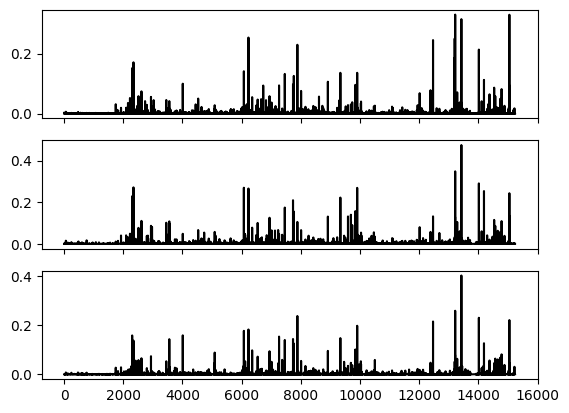
Next, we plot the vector \(p_{k,m}\) for each label \(k\).
fig, (ax1,ax2,ax3) = plt.subplots(3, 1, sharex=True)
ax1.plot(p_km[0,:], c='k')
ax2.plot(p_km[1,:], c='k')
ax3.plot(p_km[2,:], c='k')
plt.show()
We can compute a prediction on the test tweets. For example, for the 5th test tweet:
mmids.nb_predict(pi_k, p_km, X_test[4,:].toarray(), label_set)
'positive'
The following computes the overall accuracy over the test data.
acc = 0
for i in range(len(y_test)):
    if mmids.nb_predict(pi_k, p_km, X_test[i,:].toarray(), label_set) == y_test[i]:
        acc += 1
acc/(len(y_test))
0.7670765027322405
To get a better understanding of the differences uncovered by Naive Bayes between the different labels, we identify words that are particularly common in one label, but not on the other. Recall that label 1 corresponds to positive while label 2 corresponds to negative.
pos_terms = (p_km[0,:] > 0.02) & (p_km[1,:] < 0.02)
print(terms[pos_terms])
['_ù' 'amazing' 'appreciate' 'awesome' 'best' 'crew' 'first' 'flying'
 'good' 'great' 'll' 'love' 'made' 'much' 'new' 'response' 'see' 'thank'
 'thx' 'very' 'well' 'work']
One notices that many positive words do appear in this list: awesome, best, great, love, thank.
neg_terms = (p_km[1,:] > 0.02) & (p_km[0,:] < 0.02)
print(terms[neg_terms])
['about' 'after' 'again' 'agent' 'airport' 'am' 'another' 'any' 'bag'
 'bags' 'because' 'by' 'call' 'cancelled' 'change' 'check' 'days' 'delay'
 'delayed' 'did' 'don' 'due' 'even' 'ever' 'flighted' 'flightled' 'go'
 'going' 'has' 'here' 'hold' 'hour' 'hours' 'how' 'hrs' 'if' 'last' 'late'
 'lost' 'luggage' 'make' 'minutes' 'more' 'need' 'never' 'off' 'only' 'or'
 'over' 'people' 'phone' 'really' 'should' 'sitting' 'someone' 'still'
 'take' 'than' 'them' 'then' 'told' 'trying' 've' 'wait' 'waiting' 'want'
 'weather' 'what' 'when' 'why' 'worst']
This time, we notice: bag, cancelled, delayed, hours, phone.
CHAT & LEARN The bag-of-words representation used in the sentiment analysis example is a simple but limited way to represent text data. More advanced representations such as word embeddings and transformer models can capture more semantic information. Ask your favorite AI chatbot to explain these representations and how they can be used for text classification tasks. \(\ddagger\)
6.7.2.2. Kalman filtering: missing data#
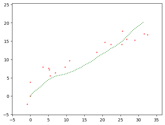
In Kalman filtering, we can also allow for the possibility that some observations are missing. Imagine for instance losing GPS signal while going through a tunnel. The recursions above are still valid, with the only modification that the Update equations involving \(\bY_t\) are dropped at those times \(t\) where there is no observation. In Numpy, we can use NaN to indicate the lack of observation. (Alternatively, one can use the numpy.ma module.)
We use a same sample path as above, but mask observations at times \(t=10,\ldots,20\).
seed = 535
rng = np.random.default_rng(seed)
ss = 4
os = 2
F = np.array([[1., 0., 1., 0.],
              [0., 1., 0., 1.],
              [0., 0., 1., 0.],
              [0., 0., 0., 1.]])
H = np.array([[1., 0., 0., 0.],
              [0., 1, 0., 0.]])
Q = 0.01 * np.diag(np.ones(ss))
R = 10 * np.diag(np.ones(os))
init_mu = np.array([0., 0., 1., 1.])
init_Sig = Q
T = 30
x, y = mmids.lgSamplePath(rng, ss, os, F, H, Q, R, init_mu, init_Sig, T)
for i in range(10,20):
    y[0,i] = np.nan
    y[1,i] = np.nan
Here is the sample we are aiming to infer.
Show code cell source
plt.scatter(y[0,:], y[1,:], s=5, c='r', alpha=0.5)
plt.plot(x[0,:], x[1,:], c='g', linestyle='dotted')
plt.xlim((np.min(x[0,:])-5, np.max(x[0,:])+5))
plt.ylim((np.min(x[1,:])-5, np.max(x[1,:])+5))
plt.show()
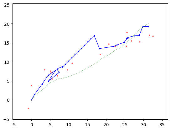
We modify the recursion accordingly, that is, skip the Update step when there is no observation to use for the update.
def kalmanUpdate(ss, F, H, Q, R, y_t, mu_prev, Sig_prev):
    mu_pred = F @ mu_prev
    Sig_pred = F @ Sig_prev @ F.T + Q
    if np.isnan(y_t[0]) or np.isnan(y_t[1]):
        return mu_pred, Sig_pred
    else:
        e_t = y_t - H @ mu_pred
        S = H @ Sig_pred @ H.T + R
        Sinv = LA.inv(S)
        K = Sig_pred @ H.T @ Sinv
        mu_new = mu_pred + K @ e_t
        Sig_new = (np.diag(np.ones(ss)) - K @ H) @ Sig_pred
        return mu_new, Sig_new
init_mu = np.array([0., 0., 1., 1.])
init_Sig = 1 * np.diag(np.ones(ss))
mu, Sig = mmids.kalmanFilter(ss, os, y, F, H, Q, R, init_mu, init_Sig, T)
Show code cell source
plt.plot(mu[0,:], mu[1,:], c='b', marker='s', markersize=2, linewidth=1)
plt.scatter(y[0,:], y[1,:], s=5, c='r', alpha=0.5)
plt.plot(x[0,:], x[1,:], c='g', linestyle='dotted', alpha=0.5)
plt.xlim((np.min(x[0,:])-5, np.max(x[0,:])+5))
plt.ylim((np.min(x[1,:])-5, np.max(x[1,:])+5))
plt.show()
6.7.2.3. Cholesky decomposition#
In this section, we derive an important matrix factorization and apply it to generating multivariate Gaussians. We also revisit the least-squares problem. We begin with the motivation.
Generating multivariate Gaussians Suppose we want to generate samples from a multivariate Gaussian \(\bX \sim N_d(\bmu, \bSigma)\) with given mean vector \(\bmu \in \mathbb{R}^d\) and positive definite covariance matrix \(\bSigma \in \mathbb{R}^{d \times d}\). Of course, in Numpy, we could use numpy.random.Generator.multivariate_normal. But what is behind it? More precisely, suppose we have access to unlimited samples \(U_1, U_2, U_3, etc.\) from uniform random variables in \([0,1]\). How do we transform them to obtain samples from \(N_d(\bmu, \bSigma)\).
We start with the simplest case: \(d=1\), \(\mu = 0\), and \(\sigma^2 = 1\). That is, we first generate a univariate standard Normal. We have seen a recipe for doing this before, the inverse transform sampling method. Specifically, recall that the cumulative distribution function (CDF) of a random variable \(Z\) is defined as
Let \(\mathcal{Z}\) be the interval where \(F_Z(z) \in (0,1)\) and assume that \(F_X\) is strictly increasing on \(\mathcal{Z}\). Let \(U \sim \mathrm{U}[0,1]\). Then it can be shown that
So take \(F_Z = \Phi\), the CDF of the standard Normal. Then \(Z = \Phi^{-1}(U)\) is \(N(0,1)\).
How do we generate a \(N(\mu, \sigma^2)\) variable, for arbitrary \(\mu \in \mathbb{R}\) and \(\sigma^2 > 0\)? We use the fact that the linear transformation of Gaussian is still Gaussian. In particular, if \(Z \sim N(0,1)\), then
is \(N(\mu, \sigma^2)\).
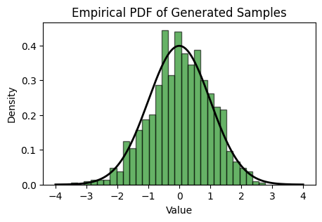
NUMERICAL CORNER: In Python, \(\Phi^{-1}\) can be accessed using scipy.stats.norm.ppf. We implement this next (with help from ChatGPT).
from scipy.stats import norm

def generate_standard_normal_samples_using_inverse_cdf(n, mu, sigma2):
    # Step 1: Generate uniform [0,1] random variables
    U = rng.uniform(0, 1, n)

    # Step 2: Apply the inverse CDF (ppf) of the standard normal distribution
    Z = norm.ppf(U)

    return mu + sigma2 * Z
We generate 1000 samples and plot the empirical distribution.
# Generate 1000 standard normal samples
samples = generate_standard_normal_samples_using_inverse_cdf(1000, 0 , 1)
Show code cell source
# Plot the empirical PDF
plt.figure(figsize=(5, 3))

# Plot histogram of the samples with density=True to normalize the histogram
count, bins, ignored = plt.hist(samples, bins=30, density=True, alpha=0.6, color='g', edgecolor='black')

# Plot the theoretical standard normal PDF for comparison
x = np.linspace(-4, 4, 1000)
plt.plot(x, norm.pdf(x), 'k', linewidth=2)

plt.title('Empirical PDF of Generated Samples')
plt.xlabel('Value')
plt.ylabel('Density')
plt.show()
\(\unlhd\)
CHAT & LEARN It turns out there is a neat trick to generate two independent samples from \(N(0,1)\) that does not rely on access to \(\Phi^{-1}\). It is called the Box-Muller transform. Ask your favorite AI chatbot about it. Modify our code above to implement it. \(\ddagger\)
We move on to the multivariate case. We proceed similarly as before. First, how do we generate a \(d\)-dimensional Gaussian with mean vector \(\bmu = \mathbf{0}\) and identity covariance matrix \(\bSigma = I_{d \times d}\)? Easy – it has \(d\) independent components, each of which is standard Normal. So letting \(U_1, \ldots, U_d\) be independent uniform \([0,1]\) variables, then
is \(N(\mathbf{0}, I_{d \times d})\).
We now seek to generate a multivariate Gaussian with arbitrary mean vector \(\bmu\) and positive definite covariance matrix \(\bSigma\). Again, we use a linear transformation
What are the right choices for \(a \in \mathbb{R}^d\) and \(A \in \mathbb{R}^{d \times d}\)? We need to match the obtained and desired mean and covariance. We start with the mean. By linearity of expectation,
Hence we pick \(\mathbf{a} := \bmu\).
As for the covariance, using the Covariance of a Linear Transformation, we get
Now we have a problem: what is a matrix \(A\) such that
In some sense, we are looking for a sort of “square root” of the covariance matrix. There are several ways of doing this. The Cholesky decomposition is one of them. We return to generating samples from \(N(\bmu, \bSigma)\) after introducing it.
A matrix factorization Our key linear-algebraic result of this section is the following. The matrix factorization in the next theorem is called a Cholesky decomposition. It has many applications.
THEOREM (Cholesky Decomposition) Any positive definite matrix \(B \in \mathbb{R}^{n \times n}\) can be factorized uniquely as
where \(L \in \mathbb{R}^{n \times n}\) is a lower triangular matrix with positive entries on the diagonal. \(\sharp\)
The proof is provided below. It is based on deriving an algorithm for computing the Cholesky decomposition: we grow \(L\) starting from its top-left corner by successively computing its next row based on the previously constructed submatrix. Note that, because \(L\) is lower triangular, it suffices to compute its elements on and below the diagonal. We first give the algorithm, then establish that it is well-defined.
Figure: Access pattern (Source)

\(\bowtie\)
EXAMPLE: Before proceeeding with the general method, we give a small example to provide some intuition as to how it operates. We need a positive definite matrix. Consider the matrix
It has full column rank (why?). Recall that, in that case, the \(B = A^T A\) is positive definite.
That is, the matrix
is positive definite.
Let \(L = (\ell_{i,j})_{i,j=1}^3\) be lower triangular. We seek to solve \(L L^T = B\) for the nonzero entries of \(L\). Observe that
The system
turns out to be fairly simple to solve.
From the first entry, we get \(\ell_{1,1} = 1\) (where we took the positive solution to \(\ell_{1,1}^2 = 1\)).
Given that \(\ell_{1,1}\) is known, entry \(\ell_{2,1}\) is determined from \(\ell_{1,1}\ell_{2,1} =2\) in the first entry of the second row. That is, \(\ell_{2,1} =2\). Then the second entry of the second row gives \(\ell_{2,2}\) through \(\ell_{2,1}^2 + \ell_{2,2}^2 = 8\). So \(\ell_{2,2} = 2\) (again we take the positive solution).
We move to the third row. The first entry gives \(\ell_{3,1} = 1\), the second entry gives \(\ell_{3,2} = -1\) and finally the third entry leads to \(\ell_{3,3} = 1\).
Hence we have
\(\lhd\)
To detail the computation of the Cholesky decomposition \(L L^T\) of \(B\), we will need some notation. Write \(B = (b_{i,j})_{i,j=1}^n\) and \(L = (\ell_{i,j})_{i,j=1}^n\). Let \(L_{(k)} = (\ell_{i,j})_{i,j=1}^k\) be the first \(k\) rows and columns of \(L\), let \(\bflambda_{(k)}^T = (\ell_{k,1},\ldots,\ell_{k,k-1})\) be the row vector corresponding to the first \(k-1\) entries of row \(k\) of \(L\), and let \(\bfbeta_{(k)}^T = (b_{k,1},\ldots,b_{k,k-1})\) be the row vector corresponding to the first \(k-1\) entries of row \(k\) of \(B\).
The strategy is to compute \(L_{(1)}\), then \(L_{(2)}\), then \(L_{(3)}\) and so on. With the notation above, \(L_{(j)}\) can be written in block form as
Hence, once \(L_{(j-1)}\) is known, in order to compute \(L_{(j)}\) one only needs \(\bflambda_{(j)}\) and \(\ell_{j,j}\). We show next that they satisfy easily solvable systems of equations.
We first note that the \((1,1)\) entry of the matrix equation \(L L^T = B\) implies that
So we set
For this step to be well-defined, it needs to be the case that \(b_{1,1} > 0\). It is easy to see that it follows from the positive definiteness of \(B\):
Proceeding by induction, assume \(L_{(j-1)}\) has been constructed. The first \(j-1\) elements of the \(j\)-th row of the matrix equation \(L L^T = B\) translate into
where \((L^T)_{\cdot,1:j-1}\) denotes the first \(j-1\) columns of \(L^T\). In the first equality above, we used the fact that \(L^T\) is upper triangular. Taking a transpose, the resulting linear system of equations
can be solved by forward substitution (since \(\bfbeta_{(j)}\) is part of the input and \(L_{(j-1)}\) was previously computed). The fact that this system has a unique solution (more specifically, that the diagonal entries of \(L_{(j-1)}\) are strictly positive) is established in the proof of the Cholesky Decomposition Theorem.
The \((j,j)\)-th entry of the matrix equation \(L L^T = B\) translates into
where again we used the fact that \(L^T\) is upper triangular. Since \(\ell_{j,1}, \ldots, \ell_{j,j-1}\) are the elements of \(\bflambda_{(j)}\), they have already been determined. So we can set
The fact that we are taking the square root of a positive quantity is established in the proof of the Cholesky Decomposition Theorem. Finally, from \(L_{(j-1)}\), \(\bflambda_{(j)}\), and \(\ell_{j,j}\), we construct \(L_{(j)}\).
NUMERICAL CORNER: We implement the algorithm above. In our naive implementation, we assume that \(B\) is positive definite, and therefore that all steps are well-defined.
def cholesky(B):
    n = B.shape[0]
    L = np.zeros((n, n))
    for j in range(n):
        L[j,0:j] = mmids.forwardsubs(L[0:j,0:j],B[j,0:j])
        L[j,j] = np.sqrt(B[j,j] - LA.norm(L[j,0:j])**2)
    return L
Here is a simple example.
B = np.array([[2., 1.],[1., 2.]])
print(B)
[[2. 1.]
 [1. 2.]]
L = cholesky(B)
print(L)
[[1.41421356 0.        ]
 [0.70710678 1.22474487]]
We can check that it produces the right factorization.
print(L @ L.T)
[[2. 1.]
 [1. 2.]]
\(\unlhd\)
Proof of Cholesky decomposition theorem We give a proof of the Cholesky Decomposition Theorem.
Proof idea: Assuming by induction that the upper-left corner of the matrix \(B\) has a Cholesky decomposition, one finds equations for the remaining row that can be solved uniquely by the properties established in the previous subsection.
Proof: If \(n=1\), we have shown previously that \(b_{1,1} > 0\), and hence we can take \(L = [\ell_{1,1}]\) where \(\ell_{1,1} = \sqrt{b_{1,1}}\). Assuming the result holds for positive definite matrices in \(\mathbb{R}^{(n-1) \times (n-1)}\), we first re-write \(B = L L^T\) in block form
where \(B_{11}, \Lambda_{11} \in \mathbb{R}^{n-1 \times n-1}\), \(\bfbeta_{12}, \bflambda_{12} \in \mathbb{R}^{n-1}\) and \(\beta_{22}, \lambda_{22} \in \mathbb{R}\). By block matrix algebra, we get the system
By the Principal Submatrices Lemma, the principal submatrix \(B_{11}\) is positive definite. Hence, by induction, there is a unique lower-triangular matrix \(\Lambda_{11}\) with positive diagonal elements satisfying the first equation. We can then obtain \(\bfbeta_{12}\) from the second equation by forward substitution. And finally we get
We do have to check that the square root above exists. That is, we need to argue that the expression inside the square root is non-negative. In fact, for the claim to go through, we need it to be strictly positive. We notice that the expression inside the square root is in fact the Schur complement of the block \(B_{11}\):
where we used the equation \(\bfbeta_{12} = \Lambda_{11} \bflambda_{12}\) on the first line, the identities \((Q W)^{-1} = W^{-1} Q^{-1}\) and \((Q^T)^{-1} = (Q^{-1})^T\) (see the exercise below) on the third line and the equation \(B_{11} = \Lambda_{11} \Lambda_{11}^T\) on the fourth line. By the Schur Complement Lemma, the Schur complement is positive definite. Because it is a scalar in this case, it is strictly positive (prove it!), which concludes the proof. \(\square\)
Back to multivariate Gaussians Returning to our motivation, we can generate samples from a \(N(\bmu, \bSigma)\) by first generating
where \(U_1, \ldots, U_d\) are independent uniform \([0,1]\) variables, then setting
where \(\bSigma = L L^T\) is a Cholesky decomposition of \(\bSigma\).
NUMERICAL CORNER: We implement this method.
def generate_multivariate_normal_samples_using_cholesky(n, d, mu, Sig):

    # Compute Cholesky decomposition
    L = cholesky(Sig)

    # Initialization
    X = np.zeros((n,d))
    for i in range(n):

            # Generate standard normal vector
            Z = generate_standard_normal_samples_using_inverse_cdf(d, 0 , 1)

            # Apply the inverse CDF (ppf) of the standard normal distribution
            X[i,:] = mu + L @ Z

    return X
We generate some samples as an example.
mu = np.array([-1.,0.,1.])
Sig = np.array([[1., 2., 1.],[2., 8., 0.],[1., 0., 3.]])
X = generate_multivariate_normal_samples_using_cholesky(10, 3, mu, Sig)
Show code cell source
print(X)
[[-0.47926185  1.97223283  2.73780609]
 [-2.69005319 -4.19788834 -0.43130768]
 [ 0.41957285  3.91719212  2.08604427]
 [-2.11532949 -5.34557983  0.69521104]
 [-2.41203356 -1.84032486 -0.82207565]
 [-1.46121329  0.4821332   0.55005982]
 [-0.84981594  0.67074839  0.16360931]
 [-2.19097155 -1.98022929 -1.06365711]
 [-2.75113597 -3.47560492 -0.26607926]
 [ 0.130848    6.07312936 -0.08800829]]
\(\unlhd\)
Using a Cholesky decomposition to solve the least squares problem Another application of the Cholesky decomposition is to solving the least squares problem. In this section, we restrict ourselves to the case where \(A \in \mathbb{R}^{n\times m}\) has full column rank. By the Least Squares and Positive Semidefiniteness Lemma, we then have that \(A^T A\) is positive definite. By the Cholesky Decomposition Theorem, we can factorize this matrix as \(A^T A = L L^T\) where \(L\) is lower triangular with positive diagonal elements. The normal equations then reduce to
This system can be solved in two steps. We first obtain the solution to
by forward substitution. Then we obtain the solution to
by back-substitution. Note that \(L^T\) is indeed an upper triangular matrix.
NUMERICAL CORNER: We implement this algorithm below. In our naive implementation, we assume that \(A\) has full column rank, and therefore that all steps are well-defined.
def ls_by_chol(A, b):
    L = cholesky(A.T @ A)
    z = mmids.forwardsubs(L, A.T @ b)
    return mmids.backsubs(L.T, z)
\(\unlhd\)
Other applications of the Cholesky decomposition are briefly described here.