2.3. The geometry of least squares: the orthogonal projection

We consider the following problem: we are given \(A \in \mathbb{R}^{n\times m}\) an \(n\times m\) matrix and \(\mathbf{b} \in \mathbb{R}^n\) a vector. We are looking to solve the system

\[ A \mathbf{x} \approx \mathbf{b}. \]

In the special case where \(A\) is invertible, a unique exact solution exists. Indeed:

DEFINITION (Nonsingular Matrix) A square matrix \(A \in \mathbb{R}^{n \times n}\) is nonsingular if it has rank \(n\). In that case, we also say that \(A\) is of full rank. \(\natural\)

THEOREM (Inverting a Nonsingular System) Let \(A \in \mathbb{R}^{n \times n}\) be a nonsingular square matrix. Then for any \(\mathbf{b} \in \mathbb{R}^n\), there exists a unique \(\mathbf{x} \in \mathbb{R}^n\) such that \(A \mathbf{x} = \mathbf{b}\). Moreover \(\mathbf{x} = A^{-1} \mathbf{b}\). \(\sharp\)

In general, however, a solution may not exist or may not be unique. We focus here on the over-determined case where the former situation generically occurs.

2.3.1. Orthogonal projection

To solve the overdetermined case, i.e., when \(n > m\), we consider the following more general problem first. We have a linear subspace \(U \subseteq \mathbb{R}^n\) and a vector \(\mathbf{v} \notin U\). We want to find the vector \(\mathbf{p}\) in \(U\) that is closest to \(\mathbf{v}\) in Euclidean norm, that is, we want to solve

\[ \min_{\mathbf{p} \in U} \|\mathbf{p} - \mathbf{v}\|. \]

EXAMPLE: Consider the two-dimensional case with a one-dimensional subspace, say \(U = \mathrm{span}(\mathbf{u_1})\) with \(\|\mathbf{u}_1\|=1\). The geometrical intuition is in the following figure. The solution \(\mathbf{p} = \mathbf{v}^*\) has the property that the difference \(\mathbf{v} - \mathbf{v}^*\) makes a right angle with \(\mathbf{u}_1\), that is, it is orthogonal to it.

Figure: Orthogonal projection on a line (Source)

\(\bowtie\)

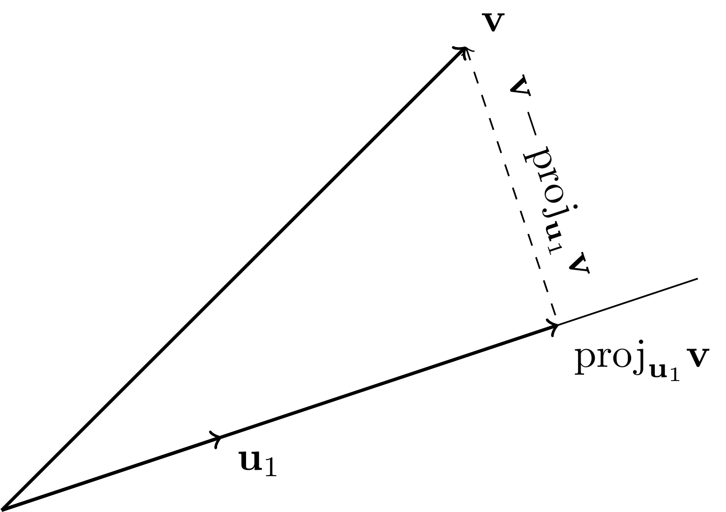
Letting \(\mathbf{v}^* = \alpha^* \,\mathbf{u}_1\), the geometrical condition above translates into

\[ 0 = \langle \mathbf{u}_1, \mathbf{v} - \mathbf{v}^* \rangle = \langle \mathbf{u}_1, \mathbf{v} - \alpha^* \,\mathbf{u}_1 \rangle = \langle \mathbf{u}_1, \mathbf{v} \rangle - \alpha^* \,\langle \mathbf{u}_1, \mathbf{u}_1 \rangle = \langle \mathbf{u}_1, \mathbf{v} \rangle - \alpha^* \]

so

\[ \mathbf{v}^* = \langle \mathbf{u}_1, \mathbf{v} \rangle \,\mathbf{u}_1. \]

By Pythagoras, we then have for any \(\alpha \in \mathbb{R}\)

\[\begin{align*} \|\mathbf{v} - \alpha \,\mathbf{u}_1\|^2 &= \|\mathbf{v}- \mathbf{v}^* + \mathbf{v}^* - \alpha \,\mathbf{u}_1\|^2\\ &= \|\mathbf{v}- \mathbf{v}^* + (\alpha^* - \alpha) \,\mathbf{u}_1\|^2\\ &= \|\mathbf{v}- \mathbf{v}^*\|^2 + \| (\alpha^* - \alpha) \,\mathbf{u}_1\|^2\\ &\geq \|\mathbf{v}- \mathbf{v}^*\|^2, \end{align*}\]

where we used that \(\mathbf{v} - \mathbf{v}^*\) is orthogonal to \(\mathbf{u}_1\) (and therefore \((\alpha^* - \alpha) \mathbf{u}_1\)) on the third line.

That confirms the optimality of \(\mathbf{v}^*\). The argument in this example carries through in higher dimension, as we show next. \(\lhd\)

DEFINITION (Orthogonal Projection on an Orthonormal List) Let \(\mathbf{q}_1,\ldots,\mathbf{q}_m\) be an orthonormal list. The orthogonal projection of \(\mathbf{v} \in \mathbb{R}^n\) on \(\{\mathbf{q}_i\}_{i=1}^m\) is defined as

\[ \mathrm{proj}_{\{\mathbf{q}_i\}_{i=1}^m} \mathbf{v} = \sum_{j=1}^m \langle \mathbf{v}, \mathbf{q}_j \rangle \,\mathbf{q}_j. \]

\(\natural\)

THEOREM (Orthogonal Projection) Let \(U \subseteq V\) be a linear subspace and let \(\mathbf{v} \in \mathbb{R}^n\). Then:

a) There exists a unique solution \(\mathbf{p}^*\) to

\[ \min_{\mathbf{p} \in U} \|\mathbf{p} - \mathbf{v}\|. \]

We denote it by \(\mathbf{p}^* = \mathrm{proj}_U \mathbf{v}\) and refer to it as the orthogonal projection of \(\mathbf{v}\) onto \(U\).

b) The solution \(\mathbf{p}^*\) is characterized geometrically by

\[ (*) \qquad \left\langle \mathbf{v} - \mathbf{p}^*, \mathbf{u}\right\rangle =0, \quad \forall \mathbf{u} \in U. \]

c) For any orthonormal basis \(\mathbf{q}_1,\ldots,\mathbf{q}_m\) of \(U\),

\[ \mathrm{proj}_U \mathbf{v} = \mathrm{proj}_{\{\mathbf{q}_i\}_{i=1}^m} \mathbf{v}. \]

\(\sharp\)

Proof: Let \(\mathbf{p}^*\) be any vector in \(U\) satisfying \((*)\). We show first that it necessarily satisfies

\[ (**) \qquad \|\mathbf{p}^* - \mathbf{v}\| \leq \|\mathbf{p} - \mathbf{v}\|, \quad \forall \mathbf{p} \in U. \]

Note that for any \(\mathbf{p} \in U\) the vector \(\mathbf{u} = \mathbf{p} - \mathbf{p}^*\) is also in \(U\). Hence by \((*)\) and Pythagoras,

\[\begin{align*} \|\mathbf{p} - \mathbf{v}\|^2 &= \|\mathbf{p} - \mathbf{p}^* + \mathbf{p}^* - \mathbf{v}\|^2\\ &= \|\mathbf{p} - \mathbf{p}^*\|^2 + \|\mathbf{p}^* - \mathbf{v}\|^2\\ &\geq \|\mathbf{p}^* - \mathbf{v}\|^2. \end{align*}\]

Furthermore, equality holds only if \(\|\mathbf{p} - \mathbf{p}^*\|^2 = 0\) which holds only if \(\mathbf{p} = \mathbf{p}^*\) by the point-separating property of the Euclidean norm. Hence, if such a vector \(\mathbf{p}^*\) exists, it is unique.

It remains to show that there is at least one vector in \(U\) satisfying \((*)\). By Gram-Schmidt, the linear subspace \(U\) has an orthonormal basis \(\mathbf{q}_1,\ldots,\mathbf{q}_m\). By definition, \(\mathrm{proj}_{\{\mathbf{q}_i\}_{i=1}^m} \mathbf{v} \in \mathrm{span}(\{\mathbf{q}_i\}_{i=1}^m) = U\). We show that \(\mathrm{proj}_{\{\mathbf{q}_i\}_{i=1}^m} \mathbf{v}\) satisfies \((*)\). We can write any \(\mathbf{u} \in U\) as \(\sum_{i=1}^m \alpha_i \mathbf{q}_i\) with \(\alpha_i = \langle \mathbf{u}, \mathbf{q}_i \rangle\). So, using this representation, we get

\[\begin{align*} \left\langle \mathbf{v} - \sum_{j=1}^m \langle \mathbf{v}, \mathbf{q}_j \rangle \,\mathbf{q}_j, \sum_{i=1}^m \alpha_i \mathbf{q}_i \right\rangle &= \sum_{j=1}^m \langle \mathbf{v}, \mathbf{q}_j \rangle \,\alpha_j - \sum_{j=1}^m \sum_{i=1}^m \alpha_i \langle \mathbf{v}, \mathbf{q}_j \rangle \langle \mathbf{q}_j, \mathbf{q}_i \rangle\\ &= \sum_{j=1}^m \langle \mathbf{v}, \mathbf{q}_j \rangle \,\alpha_j - \sum_{j=1}^m \alpha_j \langle \mathbf{v}, \mathbf{q}_j \rangle\\ &= 0, \end{align*}\]

where we used the orthonormality of the \(\mathbf{q}_j\)’s on the second line. \(\square\)

EXAMPLE: (continued) Consider again the linear subspace \(W = \mathrm{span}(\mathbf{w}_1,\mathbf{w}_2,\mathbf{w}_3)\), where \(\mathbf{w}_1 = (1,0,1)^T\), \(\mathbf{w}_2 = (0,1,1)^T\), and \(\mathbf{w}_3 = (1,-1,0)^T\). We have shown that

\[\begin{split} \mathbf{q}_1 = \frac{1}{\sqrt{2}} \begin{pmatrix} 1\\ 0\\ 1 \end{pmatrix}, \quad \mathbf{q}_2 = \frac{1}{\sqrt{6}} \begin{pmatrix} -1\\ 2\\ 1 \end{pmatrix}, \end{split}\]

is an orthonormal basis. Let \(\mathbf{w}_4 = (0,0,2)^T\). It is immediate that \(\mathbf{w}_4 \notin \mathrm{span}(\mathbf{w}_1,\mathbf{w}_2)\) since vectors in that span are of the form \((x,y,x+y)^T\) for some \(x,y \in \mathbb{R}\).

We can however compute the orthogonal projection \(\mathbf{w}_4\) onto \(W\). The inner products are

\[ \langle \mathbf{w}_4, \mathbf{q}_1 \rangle = 0 \left(\frac{1}{\sqrt{2}}\right) + 0 \left(\frac{0}{\sqrt{2}}\right) + 2 \left(\frac{1}{\sqrt{2}}\right) = \frac{2}{\sqrt{2}}, \]

\[ \langle \mathbf{w}_4, \mathbf{q}_2 \rangle = 0 \left(-\frac{1}{\sqrt{6}}\right) + 0 \left(\frac{2}{\sqrt{6}}\right) + 2 \left(\frac{1}{\sqrt{6}}\right) = \frac{2}{\sqrt{6}}. \]

So

\[\begin{split} \mathrm{proj}_W \mathbf{w}_4 = \frac{2}{\sqrt{2}} \mathbf{q}_1 + \frac{2}{\sqrt{6}} \mathbf{q}_2 = \begin{pmatrix} 2/3\\ 2/3\\ 4/3 \end{pmatrix}. \end{split}\]

As a sanity check, note that \(\mathbf{w}_4 \in W\) since its third entry is equal to the sum of its first two entries. \(\lhd\)

The map \(\mathrm{proj}_U\) is linear, that is, \(\mathrm{proj}_U (\alpha \,\mathbf{x} + \mathbf{y}) = \alpha \,\mathrm{proj}_U \mathbf{x} + \mathrm{proj}_U\mathbf{y}\) for all \(\alpha \in \mathbb{R}\) and \(\mathbf{x}, \mathbf{y} \in \mathbb{R}^n\). Indeed,

\[\begin{align*} \mathrm{proj}_U(\alpha \,\mathbf{x} + \mathbf{y}) &= \sum_{j=1}^m \langle \alpha \,\mathbf{x} + \mathbf{y}, \mathbf{q}_j \rangle \,\mathbf{q}_j\\ &= \sum_{j=1}^m \left\{\alpha \, \langle \mathbf{x}, \mathbf{q}_j \rangle + \langle \mathbf{y}, \mathbf{q}_j \rangle\right\} \mathbf{q}_j\\ &= \alpha \,\mathrm{proj}_U \mathbf{x} + \mathrm{proj}_U \mathbf{y}. \end{align*}\]

Any linear map from \(\mathbb{R}^n\) to \(\mathbb{R}^n\) can be encoded as an \(n \times n\) matrix \(P\).

Let

\[\begin{split} Q = \begin{pmatrix} | & & | \\ \mathbf{q}_1 & \ldots & \mathbf{q}_m \\ | & & | \end{pmatrix} \end{split}\]

and note that computing

\[\begin{split} Q^T \mathbf{v} = \begin{pmatrix} \langle \mathbf{v}, \mathbf{q}_1 \rangle \\ \cdots \\ \langle \mathbf{v}, \mathbf{q}_m \rangle \end{pmatrix} \end{split}\]

lists the coefficients in the expansion of \(\mathrm{proj}_U \mathbf{v}\) over the basis \(\mathbf{q}_1,\ldots,\mathbf{q}_m\).

Hence we see that

\[ P = Q Q^T. \]

Indeed, for any vector \(\mathbf{v}\),

\[ P \mathbf{v} = Q Q^T \mathbf{v} = Q [Q^T \mathbf{v}]. \]

So the output is a linear combination of the columns of \(Q\) (i.e., the \(\mathbf{q}_i\)’s) where the coefficients are the entries of the vector in square brackets \(Q^T \mathbf{v}\).

EXAMPLE: (continued) Consider again the linear subspace \(W = \mathrm{span}(\mathbf{w}_1,\mathbf{w}_2,\mathbf{w}_3)\), where \(\mathbf{w}_1 = (1,0,1)^T\), \(\mathbf{w}_2 = (0,1,1)^T\), and \(\mathbf{w}_3 = (1,-1,0)^T\), with orthonormal basis

\[\begin{split} \mathbf{q}_1 = \frac{1}{\sqrt{2}} \begin{pmatrix} 1\\ 0\\ 1 \end{pmatrix}, \quad \mathbf{q}_2 = \frac{1}{\sqrt{6}} \begin{pmatrix} -1\\ 2\\ 1 \end{pmatrix}. \end{split}\]

Then orthogonal projection onto \(W\) can be written in matrix form as follows. The matrix \(Q\) is

\[\begin{split} Q = \begin{pmatrix} 1/\sqrt{2} & -1/\sqrt{6}\\ 0 & 2/\sqrt{6}\\ 1/\sqrt{2} & 1/\sqrt{6} \end{pmatrix}. \end{split}\]

Then

\[\begin{align*} Q Q^T &= \begin{pmatrix} 1/\sqrt{2} & -1/\sqrt{6}\\ 0 & 2/\sqrt{6}\\ 1/\sqrt{2} & 1/\sqrt{6} \end{pmatrix} \begin{pmatrix} 1/\sqrt{2} & 0 & 1/\sqrt{2}\\ -1/\sqrt{6} & 2/\sqrt{6} & 1/\sqrt{6} \end{pmatrix}\\ &= \begin{pmatrix} 2/3 & -1/3 & 1/3\\ -1/3 & 2/3 & 1/3\\ 1/3 & 1/3 & 2/3 \end{pmatrix}. \end{align*}\]

So the projection of \(\mathbf{w}_4 = (0,0,2)^T\) is

\[\begin{split} \begin{pmatrix} 2/3 & -1/3 & 1/3\\ -1/3 & 2/3 & 1/3\\ 1/3 & 1/3 & 2/3 \end{pmatrix} \begin{pmatrix} 0\\ 0\\ 2 \end{pmatrix} = \begin{pmatrix} 2/3\\ 2/3\\ 4/3 \end{pmatrix}, \end{split}\]

as previously computed. \(\lhd\)

The matrix \(P= Q Q^T\) is not to be confused with

\[\begin{split} Q^T Q = \begin{pmatrix} \langle \mathbf{q}_1, \mathbf{q}_1 \rangle & \cdots & \langle \mathbf{q}_1, \mathbf{q}_m \rangle \\ \langle \mathbf{q}_2, \mathbf{q}_1 \rangle & \cdots & \langle \mathbf{q}_2, \mathbf{q}_m \rangle \\ \vdots & \ddots & \vdots \\ \langle \mathbf{q}_m, \mathbf{q}_1 \rangle & \cdots & \langle \mathbf{q}_m, \mathbf{q}_m \rangle \end{pmatrix} = I_{m \times m} \end{split}\]

where \(I_{m \times m}\) denotes the \(m \times m\) identity matrix.

EXAMPLE: Let \(\mathbf{q}_1,\ldots,\mathbf{q}_n\) be an orthonormal basis of \(\mathbb{R}^n\) and form the matrix

\[\begin{split} Q = \begin{pmatrix} | & & | \\ \mathbf{q}_1 & \ldots & \mathbf{q}_n \\ | & & | \end{pmatrix}. \end{split}\]

We show that \(Q^{-1} = Q^T\).

By the definition of matrix multiplication, recall that

\[\begin{split} Q^T Q = \begin{pmatrix} \langle \mathbf{q}_1, \mathbf{q}_1 \rangle & \cdots & \langle \mathbf{q}_1, \mathbf{q}_n \rangle \\ \langle \mathbf{q}_2, \mathbf{q}_1 \rangle & \cdots & \langle \mathbf{q}_2, \mathbf{q}_n \rangle \\ \vdots & \ddots & \vdots \\ \langle \mathbf{q}_n, \mathbf{q}_1 \rangle & \cdots & \langle \mathbf{q}_n, \mathbf{q}_n \rangle \end{pmatrix} = I_{n \times n} \end{split}\]

where \(I_{n \times n}\) denotes the \(n \times n\) identity matrix. This of course follows from the fact that the \(\mathbf{q}_i\)’s are orthonormal.

In the other direction, we claim that \(Q Q^T = I_{n \times n}\) as well. Indeed the matrix \(Q Q^T\) is the orthogonal projection on the span of the \(\mathbf{q}_i\)’s, that is, \(\mathbb{R}^n\). By the Orthogonal Projection Theorem, the orthogonal projection \(Q Q^T \mathbf{v}\) finds the closest vector to \(\mathbf{v}\) in the span of the \(\mathbf{q}_i\)’s. But that span contains all vectors, including \(\mathbf{v}\), so we must have \(Q Q^T \mathbf{v} = \mathbf{v}\). Since this holds for all \(\mathbf{v} \in \mathbb{R}^n\), the matrix \(Q Q^T\) is the identity map and we have proved the claim. \(\lhd\)

Matrices that satisfy

\[ Q^T Q = Q Q^T = I_{n \times n} \]

are called orthogonal matrices.

DEFINITION (Orthogonal Matrix) A square matrix \(Q \in \mathbb{R}^{m\times m}\) is orthogonal if \(Q^T Q = Q Q^T = I_{m \times m}\). \(\natural\)

THINK-PAIR-SHARE: Let \(\mathcal{Z}\) be a linear subspace of \(\mathbb{R}^n\) and let \(\mathbf{v} \in \mathbb{R}^n\). Show that

\[ \|\mathrm{proj}_{\mathcal{Z}}\mathbf{v}\|_2 \leq \|\mathbf{v}\|_2. \]

[Hint: Use the geometric characterization.] \(\ddagger\)

2.3.2. Orthogonal complement

Before returning to overdetermined systems, we take a little detour to derive a consequence of the orthogonal projection that will be useful later. The Orthogonal Projection Theorem implies that any \(\mathbf{v} \in \mathbb{R}^n\) can be decomposed into its orthogonal projection onto \(U\) and a vector orthogonal to it.

DEFINITION (Orthogonal Complement) Let \(U \subseteq \mathbb{R}^n\) be a linear subspace. The orthogonal complement of \(U\), denoted \(U^\perp\), is defined as

\[ U^\perp = \{\mathbf{w} \in \mathbb{R}^n\,:\, \langle \mathbf{w}, \mathbf{u}\rangle = 0, \forall \mathbf{u} \in U\}. \]

\(\natural\)

EXAMPLE: Continuing a previous example, we compute the orthogonal complement of the linear subspace \(W = \mathrm{span}(\mathbf{w}_1,\mathbf{w}_2,\mathbf{w}_3)\), where \(\mathbf{w}_1 = (1,0,1)^T\), \(\mathbf{w}_2 = (0,1,1)^T\), and \(\mathbf{w}_3 = (1,-1,0)^T\). One way to proceed is to find all vectors that are orthogonal to the orthonormal basis

\[\begin{split} \mathbf{q}_1 = \frac{1}{\sqrt{2}} \begin{pmatrix} 1\\ 0\\ 1 \end{pmatrix}, \quad \mathbf{q}_2 = \frac{1}{\sqrt{6}} \begin{pmatrix} -1\\ 2\\ 1 \end{pmatrix}. \end{split}\]

We require

\[ 0 = \langle \mathbf{u}, \mathbf{q}_1 \rangle = u_1 \left(\frac{1}{\sqrt{2}}\right) + u_2 \left(\frac{0}{\sqrt{2}}\right) + u_3 \left(\frac{1}{\sqrt{2}}\right) = \frac{u_1 + u_3}{\sqrt{2}}, \]

\[ 0= \langle \mathbf{u}, \mathbf{q}_2 \rangle = u_1 \left(-\frac{1}{\sqrt{6}}\right) + u_2 \left(\frac{2}{\sqrt{6}}\right) + u_3 \left(\frac{1}{\sqrt{6}}\right) = \frac{-u_1 + 2 u_2 + u_3}{\sqrt{6}}. \]

The first equation implies \(u_3 = -u_1\), which after replacing into the second equation and rearranging gives \(u_2 = u_1\).

So all vectors of the form \((u_1,u_1,-u_1)^T\) for some \(u_1 \in \mathbb{R}\) are orthogonal to all of \(W\). This is a one-dimensional linear subspace. We can choose an orthonormal basis by finding a solution to

\[ 1 = (u_1)^2 + (u_1)^2 + (-u_1)^2 = 3 u_1^2, \]

Take \(u_1 = 1/\sqrt{3}\), that is, let

\[\begin{split} \mathbf{q}_3 = \frac{1}{\sqrt{3}} \begin{pmatrix} 1\\ 1\\ -1 \end{pmatrix}. \end{split}\]

Then we have

\[ W^\perp = \mathrm{span}(\mathbf{q}_3). \]

\(\lhd\)

LEMMA (Orthogonal Decomposition) Let \(U \subseteq \mathbb{R}^n\) be a linear subspace and let \(\mathbf{v} \in \mathbb{R}^n\). Then \(\mathbf{v}\) can be decomposed as \(\mathrm{proj}_U \mathbf{v} + (\mathbf{v} - \mathrm{proj}_U\mathbf{v})\) where \(\mathrm{proj}_U \mathbf{v} \in U\) and \((\mathbf{v} - \mathrm{proj}_U \mathbf{v}) \in U^\perp\). Moreover, this decomposition is unique in the following sense: if \(\mathbf{v} = \mathbf{u}_1 + \mathbf{u}_2\) with \(\mathbf{u}_1 \in U\) and \(\mathbf{u}_2 \in U^\perp\), then \(\mathbf{u}_1 = \mathrm{proj}_U \mathbf{v}\) and \(\mathbf{u}_2 = \mathbf{v} - \mathrm{proj}_U \mathbf{v}\). \(\flat\)

Proof: The first part is an immediate consequence of the Orthogonal Projection Theorem. For the second part, assume \(\mathbf{v} = \mathbf{u}_1 + \mathbf{u}_2\) with \(\mathbf{u}_1 \in U\) and \(\mathbf{u}_2 \in U^\perp\). Subtracting \(\mathbf{v} = \mathrm{proj}_U \mathbf{v} + (\mathbf{v} - \mathrm{proj}_U\mathbf{v})\), we see that

\[ (*) \qquad \mathbf{0} = \mathbf{w}_1 + \mathbf{w}_2 \]

with

\[ \mathbf{w}_1 = \mathbf{u}_1 - \mathrm{proj}_U \mathbf{v} \in U, \qquad \mathbf{w}_2 = \mathbf{u}_2 - (\mathbf{v} - \mathrm{proj}_U\mathbf{v}) \in U^\perp. \]

If \(\mathbf{w}_1 = \mathbf{w}_2 = \mathbf{0}\), we are done. Otherwise, they must both be nonzero by \((*)\). Further, by the Properties of Orthonormal Lists, \(\mathbf{w}_1\) and \(\mathbf{w}_2\) must be linearly independent. But this is contradicted by the fact that \(\mathbf{w}_2 = - \mathbf{w}_1\) by \((*)\). \(\square\)

Figure: Orthogonal decomposition (Source)

\(\bowtie\)

Formally, the Orthogonal Decomposition Lemma states that \(\mathbb{R}^n\) is a direct sum of any linear subspace \(U\) and of its orthogonal complement \(U^\perp\): that is, any vector \(\mathbf{v} \in \mathbb{R}^n\) can be written uniquely as \(\mathbf{v} = \mathbf{u}_1 + \mathbf{u}_2\) with \(\mathbf{u}_1 \in U\) and \(\mathbf{u}_2 \in U^\perp\). This is denoted \(\mathbb{R}^n = U \oplus U^\perp\).

Let \(\mathbf{a}_1,\ldots,\mathbf{a}_\ell\) be an orthonormal basis of \(U\) and \(\mathbf{b}_1,\ldots,\mathbf{b}_k\) be an orthonormal basis of \(U^\perp\). By definition of the orthogonal complement, the list

\[ \mathcal{L} = \{\mathbf{a}_1,\ldots,\mathbf{a}_\ell, \mathbf{b}_1,\ldots,\mathbf{b}_k\} \]

is orthonormal, so it forms a basis of its span. Because any vector in \(\mathbb{R}^n\) can be written as a sum of a vector from \(U\) and a vector from \(U^\perp\), all of \(\mathbb{R}^n\) is in the span of \(\mathcal{L}\). It follows from the Dimension Theorem that \(n = \ell + k\), that is,

\[ \mathrm{dim}(U) + \mathrm{dim}(U^\perp) = n. \]

2.3.3. Overdetermined systems

In this section, we discuss the least-squares problem. Let again \(A \in \mathbb{R}^{n\times m}\) be an \(n\times m\) matrix with linearly independent columns and let \(\mathbf{b} \in \mathbb{R}^n\) be a vector. We are looking to solve the system

\[ A \mathbf{x} \approx \mathbf{b}. \]

If \(n=m\), we can use the matrix inverse to solve the system, as discussed in the previous subsection. But we are particularly interested in the overdetermined case, i.e. when \(n > m\): there are more equations than variables. We cannot use the matrix inverse then. Indeed, because the columns do not span all of \(\mathbb{R}^n\), there is a vector \(\mathbf{b} \in \mathbb{R}^n\) that is not in the column space of \(A\).

A natural way to make sense of the overdetermined problem is to cast it as the linear least squares problem

\[ \min_{\mathbf{x} \in \mathbb{R}^m} \|A \mathbf{x} - \mathbf{b}\|. \]

In words, we look for the best-fitting solution under the Euclidean norm. Equivalently, writing

\[\begin{split} A = \begin{pmatrix} | & & | \\ \mathbf{a}_1 & \ldots & \mathbf{a}_m \\ | & & | \end{pmatrix} = \begin{pmatrix} a_{11} & \cdots & a_{1m} \\ a_{21} & \cdots & a_{2m} \\ \vdots & \ddots & \vdots \\ a_{n1} & \cdots & a_{nm} \end{pmatrix} \quad \text{and} \quad \mathbf{b} = \begin{pmatrix} b_1 \\ \vdots \\ b_n \end{pmatrix} \end{split}\]

we seek a linear combination of the columns of \(A\) that minimizes the objective

\[ \left\|\,\sum_{j=1}^m x_j \mathbf{a}_j - \mathbf{b}\,\right\|^2 = \sum_{i=1}^n \left( \sum_{j=1}^m a_{ij} x_j - b_i \right)^2. \]

We have already solved a closely related problem when we introduced the orthogonal projection. We make the connection explicit next.

THEOREM (Normal Equations) Let \(A \in \mathbb{R}^{n\times m}\) be an \(n\times m\) matrix with \(n \geq m\) and let \(\mathbf{b} \in \mathbb{R}^n\) be a vector. A solution \(\mathbf{x}^*\) to the linear least squares problem

\[ \min_{\mathbf{x} \in \mathbb{R}^m} \|A \mathbf{x} - \mathbf{b}\| \]

satisfies the normal equations

\[ A^T A \mathbf{x}^* = A^T \mathbf{b}. \]

If further the columns of \(A\) are linearly independent, then there exists a unique solution \(\mathbf{x}^*\). \(\sharp\)

Proof idea: Apply our characterization of the orthogonal projection onto the column space of \(A\).

Proof: Let \(U = \mathrm{col}(A) = \mathrm{span}(\mathbf{a}_1,\ldots,\mathbf{a}_m)\). By the Orthogonal Projection Theorem, the orthogonal projection \(\mathbf{p}^* = \mathrm{proj}_{U} \mathbf{b}\) of \(\mathbf{b}\) onto \(U\) is the unique, closest vector to \(\mathbf{b}\) in \(U\), that is,

\[ \mathbf{p}^* = \arg\min_{\mathbf{p} \in U} \|\mathbf{p} - \mathbf{b}\|. \]

Because \(\mathbf{p}^*\) is in \(U = \mathrm{col}(A)\), it must be of the form \(\mathbf{p}^* = A \mathbf{x}^*\). This establishes that \(\mathbf{x}^*\) is a solution to the linear least squares problem in the statement.

Important observation: while we have shown that \(\mathbf{p}^*\) is unique (by the Orthogonal Projection Theorem), it is not clear at all that \(\mathbf{x}^*\) (i.e., the linear combination of columns of \(A\) corresponding to \(\mathbf{p}^*\)) is unique. By the Orthogonal Projection Theorem, it must satisfy \(\langle \mathbf{b} - A \mathbf{x}^*, \mathbf{u}\rangle = 0\) for all \(\mathbf{u} \in U\). Because the columns \(\mathbf{a}_i\) are in \(U\), that implies that

\[ 0 = \langle \mathbf{b} - A \mathbf{x}^*, \mathbf{a}_i\rangle = \mathbf{a}_i^T (\mathbf{b} - A \mathbf{x}^*) ,\qquad \forall i\in [m]. \]

Stacking up these equations gives in matrix form

\[ A^T (\mathbf{b} - A\mathbf{x}^*) = \mathbf{0}, \]

as claimed.

We have seen in a previous example that, when \(A\) has full column rank, the matrix \(A^T A\) is invertible. That implies the uniqueness claim. \(\square\)

NUMERICAL CORNER: To solve a linear system in Numpy, use numpy.linalg.solve. As an example, we consider the overdetermined system with

\[\begin{split} A = \begin{pmatrix} 1 & 0\\ 0 & 1\\ 1 & 1 \end{pmatrix} \quad \text{and} \quad \mathbf{b} = \begin{pmatrix} 0\\ 0\\ 2 \end{pmatrix}. \end{split}\]

We use numpy.ndarray.T for the transpose.

w1 = np.array([1., 0., 1.])
w2 = np.array([0., 1., 1.])
A = np.stack((w1, w2),axis=-1)
b = np.array([0., 0., 2.])
x = LA.solve(A.T @ A, A.T @ b)
print(x)

[0.66666667 0.66666667]

We can also use numpy.linalg.lstsq directly on the overdetermined system to compute the least-square solution.

x = LA.lstsq(A, b, rcond=None)[0]
print(x)

[0.66666667 0.66666667]

\(\unlhd\)