\(\newcommand{\bmu}{\boldsymbol{\mu}}\) \(\newcommand{\bSigma}{\boldsymbol{\Sigma}}\) \(\newcommand{\bfbeta}{\boldsymbol{\beta}}\) \(\newcommand{\bflambda}{\boldsymbol{\lambda}}\) \(\newcommand{\bgamma}{\boldsymbol{\gamma}}\) \(\newcommand{\bsigma}{{\boldsymbol{\sigma}}}\) \(\newcommand{\bpi}{\boldsymbol{\pi}}\) \(\newcommand{\btheta}{{\boldsymbol{\theta}}}\) \(\newcommand{\bphi}{\boldsymbol{\phi}}\) \(\newcommand{\balpha}{\boldsymbol{\alpha}}\) \(\newcommand{\blambda}{\boldsymbol{\lambda}}\) \(\renewcommand{\P}{\mathbb{P}}\) \(\newcommand{\E}{\mathbb{E}}\) \(\newcommand{\indep}{\perp\!\!\!\perp} \newcommand{\bx}{\mathbf{x}}\) \(\newcommand{\bp}{\mathbf{p}}\) \(\renewcommand{\bx}{\mathbf{x}}\) \(\newcommand{\bX}{\mathbf{X}}\) \(\newcommand{\by}{\mathbf{y}}\) \(\newcommand{\bY}{\mathbf{Y}}\) \(\newcommand{\bz}{\mathbf{z}}\) \(\newcommand{\bZ}{\mathbf{Z}}\) \(\newcommand{\bw}{\mathbf{w}}\) \(\newcommand{\bW}{\mathbf{W}}\) \(\newcommand{\bv}{\mathbf{v}}\) \(\newcommand{\bV}{\mathbf{V}}\) \(\newcommand{\bfg}{\mathbf{g}}\) \(\newcommand{\bfh}{\mathbf{h}}\) \(\newcommand{\horz}{\rule[.5ex]{2.5ex}{0.5pt}}\) \(\renewcommand{\S}{\mathcal{S}}\) \(\newcommand{\X}{\mathcal{X}}\) \(\newcommand{\var}{\mathrm{Var}}\) \(\newcommand{\pa}{\mathrm{pa}}\) \(\newcommand{\Z}{\mathcal{Z}}\) \(\newcommand{\bh}{\mathbf{h}}\) \(\newcommand{\bb}{\mathbf{b}}\) \(\newcommand{\bc}{\mathbf{c}}\) \(\newcommand{\cE}{\mathcal{E}}\) \(\newcommand{\cP}{\mathcal{P}}\) \(\newcommand{\bbeta}{\boldsymbol{\beta}}\) \(\newcommand{\bLambda}{\boldsymbol{\Lambda}}\) \(\newcommand{\cov}{\mathrm{Cov}}\) \(\newcommand{\bfk}{\mathbf{k}}\) \(\newcommand{\idx}[1]{}\) \(\newcommand{\xdi}{}\)

8.1. Motivating example: classifying natural images

In this chapter, we return to the classification problem. This time we consider more complex datasets involving natural images. We have seen an example previously, the MNIST dataset. We use a related dataset known as Fashion-MNIST developed by the Zalando Research. Quoting from their GitHub repository:

Fashion-MNIST is a dataset of Zalando’s article images – consisting of a training set of 60,000 examples and a test set of 10,000 examples. Each example is a 28x28 grayscale image, associated with a label from 10 classes. We intend Fashion-MNIST to serve as a direct drop-in replacement for the original MNIST dataset for benchmarking machine learning algorithms. It shares the same image size and structure of training and testing splits.

Figure: Fashion-MNIST sample images (Source)

\(\bowtie\)

We first load the data and convert it to an appropriate matrix representation. The data can be accessed with torchvision.datasets.FashionMNIST.

import torch
from torchvision import datasets, transforms
from torch.utils.data import DataLoader, TensorDataset

fashion_mnist = datasets.FashionMNIST(root='./data', train=True, 
                                      download=True, transform=transforms.ToTensor())

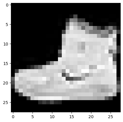
For example, the first image and its label are the following. The squeeze() below removes the color dimension in the image, which is grayscale.

img, label = fashion_mnist[0]
plt.figure()
plt.imshow(img.squeeze(), cmap='gray')
plt.show()

label

9

This label is not particularly meaningful. One can get the actual names of the classes as follows.

def FashionMNIST_get_class_name(label):

    class_names = ["T-shirt/top", "Trouser", "Pullover", "Dress", 
    "Coat", "Sandal", "Shirt", "Sneaker", "Bag", "Ankle boot"]

    return class_names[label]

print(f"{label}: '{FashionMNIST_get_class_name(label)}'")

9: 'Ankle boot'

The purpose of this chapter is to develop some of the mathematical tools used to solve this kind of classification problem:

• neural networks,

• backpropagation,

• stochastic gradient descent.