
\(\newcommand{\bmu}{\boldsymbol{\mu}}\) \(\newcommand{\bSigma}{\boldsymbol{\Sigma}}\) \(\newcommand{\bfbeta}{\boldsymbol{\beta}}\) \(\newcommand{\bflambda}{\boldsymbol{\lambda}}\) \(\newcommand{\bgamma}{\boldsymbol{\gamma}}\) \(\newcommand{\bsigma}{{\boldsymbol{\sigma}}}\) \(\newcommand{\bpi}{\boldsymbol{\pi}}\) \(\newcommand{\btheta}{{\boldsymbol{\theta}}}\) \(\newcommand{\bphi}{\boldsymbol{\phi}}\) \(\newcommand{\balpha}{\boldsymbol{\alpha}}\) \(\newcommand{\blambda}{\boldsymbol{\lambda}}\) \(\renewcommand{\P}{\mathbb{P}}\) \(\newcommand{\E}{\mathbb{E}}\) \(\newcommand{\indep}{\perp\!\!\!\perp} \newcommand{\bx}{\mathbf{x}}\) \(\newcommand{\bp}{\mathbf{p}}\) \(\renewcommand{\bx}{\mathbf{x}}\) \(\newcommand{\bX}{\mathbf{X}}\) \(\newcommand{\by}{\mathbf{y}}\) \(\newcommand{\bY}{\mathbf{Y}}\) \(\newcommand{\bz}{\mathbf{z}}\) \(\newcommand{\bZ}{\mathbf{Z}}\) \(\newcommand{\bw}{\mathbf{w}}\) \(\newcommand{\bW}{\mathbf{W}}\) \(\newcommand{\bv}{\mathbf{v}}\) \(\newcommand{\bV}{\mathbf{V}}\) \(\newcommand{\bfg}{\mathbf{g}}\) \(\newcommand{\bfh}{\mathbf{h}}\) \(\newcommand{\horz}{\rule[.5ex]{2.5ex}{0.5pt}}\) \(\renewcommand{\S}{\mathcal{S}}\) \(\newcommand{\X}{\mathcal{X}}\) \(\newcommand{\var}{\mathrm{Var}}\) \(\newcommand{\pa}{\mathrm{pa}}\) \(\newcommand{\Z}{\mathcal{Z}}\) \(\newcommand{\bh}{\mathbf{h}}\) \(\newcommand{\bb}{\mathbf{b}}\) \(\newcommand{\bc}{\mathbf{c}}\) \(\newcommand{\cE}{\mathcal{E}}\) \(\newcommand{\cP}{\mathcal{P}}\) \(\newcommand{\bbeta}{\boldsymbol{\beta}}\) \(\newcommand{\bLambda}{\boldsymbol{\Lambda}}\) \(\newcommand{\cov}{\mathrm{Cov}}\) \(\newcommand{\bfk}{\mathbf{k}}\) \(\newcommand{\idx}[1]{}\) \(\newcommand{\xdi}{}\)
2.1. Motivating example: predicting sales#
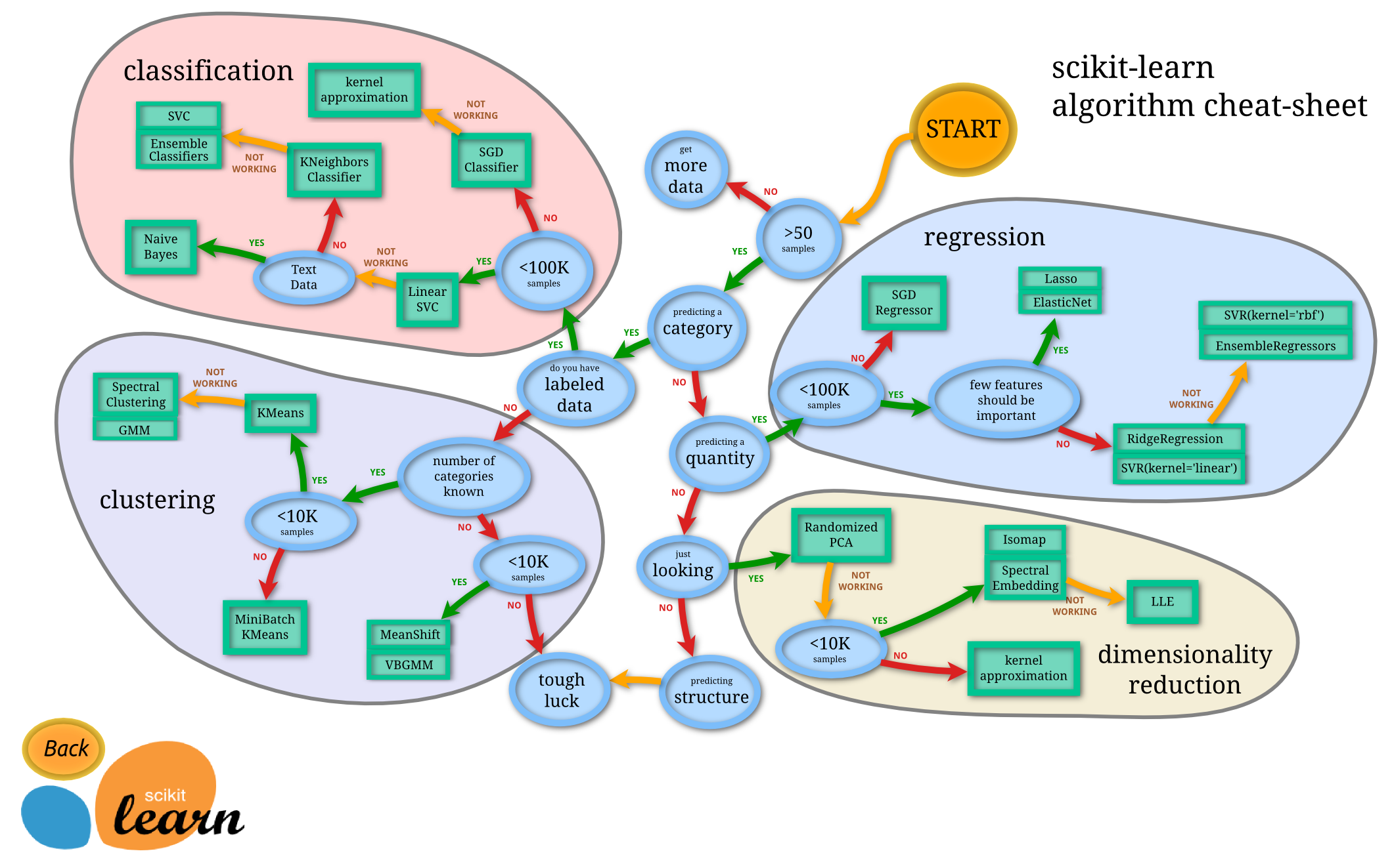
Figure: Helpful map of ML by scitkit-learn (Source)
\(\bowtie\)
The following dataset is from the excellent textbook [ISLP]. Quoting [ISLP, Section 2.1]:
Suppose that we are statistical consultants hired by a client to provide advice on how to improve sales of a particular product. The
advertisingdata set consists of thesalesof that product in 200 different markets, along with advertising budgets for the product in each of those markets for three different media:TV,radio, andnewspaper. […] It is not possible for our client to directly increase sales of the product. On the other hand, they can control the advertising expenditure in each of the three media. Therefore, if we determine that there is an association between advertising and sales, then we can instruct our client to adjust advertising budgets, thereby indirectly increasing sales. In other words, our goal is to develop an accurate model that can be used to predict sales on the basis of the three media budgets.
This a regression problem. That is, we want to estimate the relationship between an outcome variable and one or more predictors (or features). We load the data.
data = pd.read_csv('advertising.csv')
data.head()
| TV | radio | newspaper | sales | |
|---|---|---|---|---|
| 0 | 230.1 | 37.8 | 69.2 | 22.1 |
| 1 | 44.5 | 39.3 | 45.1 | 10.4 |
| 2 | 17.2 | 45.9 | 69.3 | 9.3 |
| 3 | 151.5 | 41.3 | 58.5 | 18.5 |
| 4 | 180.8 | 10.8 | 58.4 | 12.9 |
We will focus for now on the TV budget.
TV = data['TV'].to_numpy()
sales = data['sales'].to_numpy()
We make a scatterplot showing the relation between those two quantities.
plt.scatter(TV, sales, s=5, c='k')
plt.xlabel('TV'), plt.ylabel('sales')
plt.show()
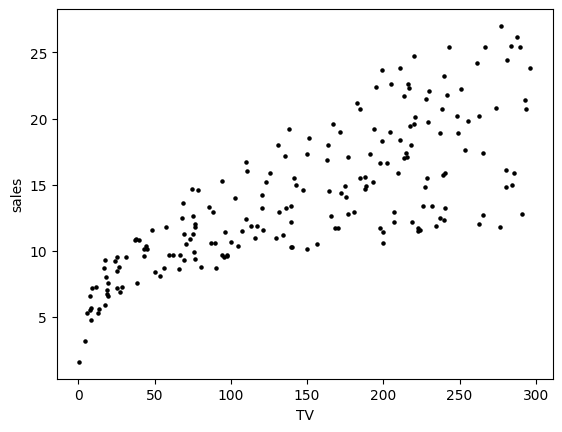
There does seem to be a relationship between the two. Roughly a higher TV budget is linked to higher sales, although the correspondence is not perfect. To express the relationship more quantitatively, we seek a function \(f\) such that
where \(x\) denotes a sample TV budget and \(y\) is the corresponding observed sales. We might posit for instance that there exists a true \(f\) and that each observation is disrupted by some noise \(\varepsilon\)
A natural way to estimate such an \(f\) from data is \(k\)-nearest-neighbors (\(k\)-NN) regression\(\idx{k-NN regression}\xdi\). Let the data be of the form \(\{(\mathbf{x}_i, y_i)\}_{i=1}^n\) where \(\mathbf{x}_i \in \mathbb{R}^d\) and \(y_i \in \mathbb{R}\). In our case \(\mathbf{x}_i\) is the (real-valued) TV budget of the \(i\)-th sample (so \(d=1\)) and \(y_i\) is the corresponding sales. For each \(\mathbf{x}\) (not necessarily in the data), we do the following:
find the \(k\) nearest \(\mathbf{x}_i\)’s to \(\mathbf{x}\)
take an average of the corresponding \(y_i\)’s.
We implement this method in Python. We use the function numpy.argsort to sort an array and the function numpy.absolute to compute the absolute deviation. Our quick implementation here assumes that the \(\mathbf{x}_i\)’s are scalars.
def knnregression(x,y,k,xnew):
    n = len(x)
    closest = np.argsort([np.absolute(x[i]-xnew) for i in range(n)])
    return np.mean(y[closest[0:k]])
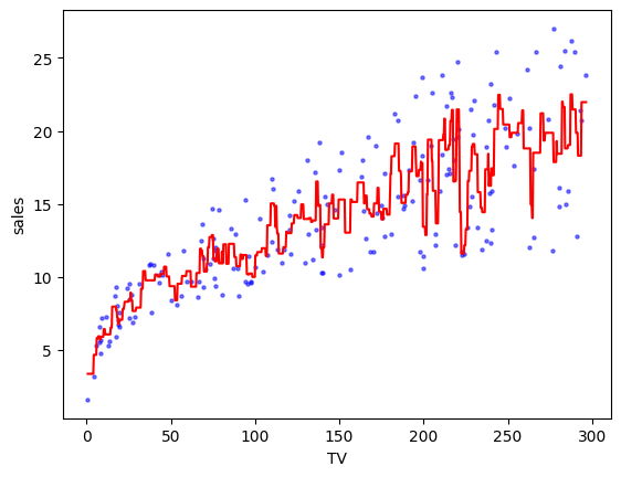
For \(k=3\) and a grid of \(1000\) points, we get the following approximation \(\hat{f}\). Here the function numpy.linspace creates an array of equally spaced points.
k = 3
xgrid = np.linspace(TV.min(), TV.max(), num=1000)
yhat = [knnregression(TV,sales,k,xnew) for xnew in xgrid]

plt.scatter(TV, sales, s=5, c='b', alpha=0.5)
plt.plot(xgrid, yhat, 'r')
plt.xlabel('TV'), plt.ylabel('sales')
plt.show()
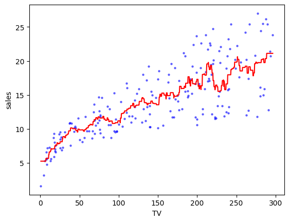
A higher \(k\) produces something less wiggly.
k = 10
xgrid = np.linspace(TV.min(), TV.max(), num=1000)
yhat = [knnregression(TV,sales,k,xnew) for xnew in xgrid]

plt.scatter(TV, sales, s=5, c='b', alpha=0.5)
plt.plot(xgrid, yhat, 'r')
plt.xlabel('TV'), plt.ylabel('sales')
plt.show()
One downside of \(k\)-NN regression is that it does not give an easily interpretable relationship: if I increase my TV budget by \(\Delta\) dollars, how is it expected to affect the sales? Another issue arises in high dimension where the counter-intuitive phenomena we discussed in a previous section can have a significant impact. Recall in particular the High-dimensional Cube Theorem. If we have \(d\) predictors – where \(d\) is large – and our data is distributed uniformly in a bounded region, then any given \(\mathbf{x}\) will be far from any of our data points. In that case, the \(y\)-values of the closest \(\mathbf{x}_i\)’s may not be predictive. This is referred to as the Curse of Dimensionality\(\idx{curse of dimensionality}\xdi\).
CHAT & LEARN Ask your favorite AI chatbot for more details on the Curse of Dimensionality and how it arises in data science. \(\ddagger\)
One way out is to make stronger assumptions on the function \(f\). For instance, we can assume that the true relationship is (approximately) affine, that is, \(y \approx \beta_0 + \beta_1 x\), or if we have \(d\) predictors
How do we estimate appropriate intercept and coefficients? The standard approach is to minimize the sum of the squared errors
where \((\mathbf{x}_{i})_j\) is the \(j\)-th entry of input vector \(\mathbf{x}_i \in \mathbb{R}^d\) and \(y_i \in \mathbb{R}\) is the corresponding \(y\)-value. This is called multiple linear regression.
It is a least-squares problem. We re-write it in a more convenient matrix form and combine \(\beta_0\) with the other \(\beta_i\)’s by adding a dummy predictor to each sample. Let
Then observe that
The linear least-squares problem is then formulated as
In words, we are looking for a linear combination of the columns of \(A\) that is closest to \(\mathbf{y}\) in Euclidean distance. Indeed, minimizing the squared Euclidean distance is equivalent to minimizing its square root, as the latter in an increasing function.
One could solve this optimization problem through calculus (and we will come back to this approach later in the book), but understanding the geometric and algebraic structure of the problem turns out to provide powerful insights into its solution – and that of many of problems in data science. It will also be an opportunity to review some basic linear-algebraic concepts along the way.
We will come back to the advertising dataset later in the chapter.