Exercises

$\newcommand{\P}{\mathbb{P}}$ $\newcommand{\E}{\mathbb{E}}$ $\newcommand{\S}{\mathcal{S}}$ $\newcommand{\var}{\mathrm{Var}}$ $\newcommand{\bmu}{\boldsymbol{\mu}}$ $\newcommand{\bSigma}{\boldsymbol{\Sigma}}$ $\newcommand{\btheta}{\boldsymbol{\theta}}$ $\newcommand{\bpi}{\boldsymbol{\pi}}$ $\newcommand{\indep}{\perp\!\!\!\perp}$ $\newcommand{\bp}{\mathbf{p}}$ $\newcommand{\bx}{\mathbf{x}}$ $\newcommand{\bX}{\mathbf{X}}$ $\newcommand{\by}{\mathbf{y}}$ $\newcommand{\bY}{\mathbf{Y}}$ $\newcommand{\bz}{\mathbf{z}}$ $\newcommand{\bZ}{\mathbf{Z}}$ $\newcommand{\bw}{\mathbf{w}}$ $\newcommand{\bW}{\mathbf{W}}$ $\newcommand{\bv}{\mathbf{v}}$ $\newcommand{\bV}{\mathbf{V}}$ $\newcommand{\Z}{\mathcal{Z}}$ $\newcommand{\bphi}{\boldsymbol{\phi}}$

6.6. Exercises#

6.6.1. Warm-up worksheets#

(with help from Claude, Gemini, and ChatGPT)

Section 6.2

E6.2.1 For a categorical random variable $Y$ with $K = 3$ categories and probabilities $\pi_1 = 0.2$, $\pi_2 = 0.5$, and $\pi_3 = 0.3$, compute the probability $\mathbb{P}(Y = e_2)$.

E6.2.2 Given a dataset of 10 coin flips $(1, 0, 1, 1, 0, 0, 1, 1, 0, 1)$, find the maximum likelihood estimate of the parameter $q$ of a Bernoulli distribution.

E6.2.3 Prove that the maximum likelihood estimator for the parameter of a Bernoulli distribution is statistically consistent.

E6.2.4 Given a dataset $\{(x_i, y_i)\}_{i=1}^n$ with $x_i \in \mathbb{R}$ and $y_i \in \{0, 1\}$, write down the negative log-likelihood for logistic regression and compute its gradient.

E6.2.5 For the dataset $\{(1, 1), (2, 0), (3, 1), (4, 0)\}$, perform one step of gradient descent for logistic regression with learning rate $\eta = 0.1$ and initial parameter $w = 0$.

E6.2.6 Compute the gradient and Hessian of the negative log-likelihood for a generalized linear model with a Poisson distribution with mean $\lambda$.

E6.2.7 A discrete random variable $X$ has probability mass function (PMF) given by

\[ P(X = x) = \frac{1}{Z(\theta)} h(x) \exp(\theta x), \]

where $x \in \{-1, 0, 1\}$. Find the value of $Z(\theta)$.

E6.2.8 Let $X$ be a random variable with probability mass function (PMF) given by

\[ P(X = x) = \frac{1}{Z(\theta)} \exp(\theta x^2), \]

where $x \in \{-1, 0, 1\}$. Find the partition function $Z(\theta)$.

E6.2.9 Given the sample $\{X_1 = 1, X_2 = 2, X_3 = 2, X_4 = 3\}$ from a multinomial distribution with $n = 4$ trials and $K = 3$ categories, compute the empirical frequency for each category.

E6.2.10 Compute the determinant of the covariance matrix $\Sigma = \begin{pmatrix} 4 & 2 \\ 2 & 3 \end{pmatrix}$.

E6.2.11 For a multivariate Gaussian vector $X \in \mathbb{R}^2$ with mean $\mu = \begin{pmatrix} 1 \\ 2 \end{pmatrix}$ and covariance matrix $\Sigma = \begin{pmatrix} 2 & 1 \\ 1 & 2 \end{pmatrix}$, compute the log-likelihood of observing $X = \begin{pmatrix} 1 \\ 3 \end{pmatrix}$.

Section 6.3

E6.3.1 Given the events $A$ and $B$ with $P(A) = 0.4$, $P(B) = 0.5$, and $P(A \cap B) = 0.2$, compute the conditional probability $P(A|B)$.

E6.3.2 Given the random variables $X$ and $Y$ with joint probability mass function $p_{X,Y}(x,y) = \frac{1}{4}$ for $x, y \in \{0, 1\}$, find $P(Y=1|X=0)$.

E6.3.3 Calculate the conditional expectation $\mathbb{E}[X|Y=y]$ for a discrete random variable $X$ with $\mathbb{P}(X = 1|Y = y) = 0.3$ and $\mathbb{P}(X = 2|Y = y) = 0.7$.

E6.3.4 For the events $A$ and $B$ with $P(A|B) = 0.6$ and $P(B) = 0.5$, calculate $P(A \cap B)$.

E6.3.5 Given events $A$, $B$, and $C$ with $P[A] = 0.6$, $P[B] = 0.5$, $P[C] = 0.4$, $P[A \cap B] = 0.3$, $P[A \cap C] = 0.2$, $P[B \cap C] = 0.1$, and $P[A \cap B \cap C] = 0.05$, compute $P[A \mid B \cap C]$.

E6.3.6 Given events $A$, $B$, and $C$ with $P[A] = 0.7$, $P[B \mid A] = 0.6$, and $P[C \mid A \cap B] = 0.4$, compute $P[A \cap B \cap C]$.

E6.3.7 Given events $A$, $B$, and $C$ with $P[A] = 0.8$, $P[B] = 0.6$, and $P[C] = 0.5$, and assuming that $A$, $B$, and $C$ are pairwise independent, compute $P[A \cap B \cap C]$.

E6.3.8 Let $X, Y, Z$ be random variables taking values in $\{0,1\}$. Given a fork configuration $Y \leftarrow X \rightarrow Z$ with $(P[X=x])_{x} = (0.2, 0.8)$, $P([Y=y \mid X=x])_{x,y} = \begin{pmatrix} 0.6 & 0.4 \\ 0.3 & 0.7 \end{pmatrix}$, and $(P[Z=z \mid X=x])_{x,z} = \begin{pmatrix} 0.8 & 0.2 \\ 0.1 & 0.9 \end{pmatrix}$, compute $(P[Y=y, Z=z])_{y,z}$.

E6.3.9 Let $X, Y, Z$ be random variables taking values in $\{0,1\}$. Given a chain configuration $X \rightarrow Y \rightarrow Z$ with $(P[X=x])_x = (0.3, 0.7)$, $(P[Y=y \mid X=x])_{x,y} = \begin{pmatrix} 0.2 & 0.8 \\ 0.6 & 0.4 \end{pmatrix}$, and $(P[Z=z \mid Y=y])_{y,z} = \begin{pmatrix} 0.5 & 0.5 \\ 0.1 & 0.9 \end{pmatrix}$, compute $(P[X=x, Z=z])_{x,z}$.

E6.3.10 Consider a document classification problem with a vocabulary of 4 words and 2 topics. Given $\pi = (0.5, 0.5)$, $p_1 = (0.1, 0.5, 0.1, 0.5)$, and $p_2 = (0.5, 0.5, 0.1, 0.1)$, compute $P[C = 1, X = (1, 0, 1, 0)]$.

E6.3.11 Consider a document classification problem with a vocabulary of 3 words and 2 topics. Given a training dataset with $N_{1,1} = 10$, $N_{1,2} = 20$, $N_{1,3} = 20$, $N_{2,1} = 40$, $N_{2,2} = 30$, and $N_{2,3} = 30$, compute the maximum likelihood estimates of $\pi_1$, $p_{1,1}$, and $p_{2,1}$.

E6.3.12 Suppose $A$, $B$, and $C$ are events such that $P[C] > 0$ and $A \indep B | C$. If $P[A|C] = 0.3$ and $P[B|C] = 0.6$, calculate $P[A \cap B | C]$.

E6.3.13 Consider the following graphical model:

G = nx.DiGraph()
G.add_edges_from([("X", "Y"), ("X", "Z")])

Write down the joint probability distribution $P[X=x, Y=y, Z=z]$ using the chain rule of probability.

E6.3.14 In the Naive Bayes model, if a document contains the words “love” and “great,” and the model parameters are $p_{1,\text{love}} = 0.8$, $p_{1,\text{great}} = 0.7$, $p_{2,\text{love}} = 0.2$, and $p_{2,\text{great}} = 0.3$, which class (1 or 2) is the document more likely to belong to?

Section 6.4

E6.4.1 Let $X$ be a random variable that follows a mixture of two Bernoulli distributions with parameters $p_1 = 0.3$ and $p_2 = 0.8$, and mixing weights $\pi_1 = 0.6$ and $\pi_2 = 0.4$. Compute $P(X = 1)$.

E6.4.2 In a Gaussian Mixture Model (GMM) with two components, suppose $\boldsymbol{\mu}_1 = (1, 2)$, $\boldsymbol{\mu}_2 = (-1, -1)$, $\Sigma_1 = \Sigma_2 = I_{2 \times 2}$, and $\pi_1 = \pi_2 = 0.5$. Write down the probability density function of this GMM.

E6.4.3 Given a mixture of two multivariate Bernoulli distributions with parameters $\pi_1 = 0.4$, $\pi_2 = 0.6$, $p_{1,1} = 0.7$, $p_{1,2} = 0.3$, $p_{2,1} = 0.2$, and $p_{2,2} = 0.8$, compute the probability of observing the data point $x = (1, 0)$.

E6.4.4 Given a mixture of two univariate Gaussian distributions with parameters $\pi_1 = 0.3$, $\pi_2 = 0.7$, $\mu_1 = 1$, $\mu_2 = 4$, $\sigma_1^2 = 1$, and $\sigma_2^2 = 2$, compute the probability density function (PDF) at $x = 2$.

E6.4.5 Given a mixture of two multivariate Bernoulli distributions with parameters $\pi_1 = 0.5$, $\pi_2 = 0.5$, $p_{1,1} = 0.8$, $p_{1,2} = 0.2$, $p_{2,1} = 0.1$, and $p_{2,2} = 0.9$, compute the responsibilities $r_{1,i}$ and $r_{2,i}$ for the data point $x_i = (1, 1)$.

E6.4.6 Given a mixture of two univariate Gaussian distributions with parameters $\pi_1 = 0.4$, $\pi_2 = 0.6$, $\mu_1 = 2$, $\mu_2 = 5$, $\sigma_1^2 = 1$, and $\sigma_2^2 = 2$, and a data point $x = 3$, compute the responsibilities $r_{1}$ and $r_{2}$.

E6.4.7 Given a mixture of two multivariate Bernoulli distributions with parameters $\pi_1 = 0.6$, $\pi_2 = 0.4$, and responsibilities $r_{1,1} = 0.8$ and $r_{2,2} = 0.2$ for data points $x_1 = (1, 0)$ and $x_2 = (0, 1)$, update the parameters $\pi_1$ and $\pi_2$ using the M-step of the EM algorithm.

E6.4.8 Given a mixture of two univariate Gaussian distributions with parameters $\pi_1 = 0.5$, $\pi_2 = 0.5$, responsibilities $r_{1,1} = 0.7$, $r_{2,1} = 0.3$, and data points $x_1 = 1$ and $x_2 = 4$, update the means $\mu_1$ and $\mu_2$ using the M-step of the EM algorithm.

E6.4.9 In the EM algorithm for mixtures of multivariate Bernoullis, suppose you have three data points: $\mathbf{x}_1 = (1, 0, 1)$, $\mathbf{x}_2 = (0, 1, 0)$, and $\mathbf{x}_3 = (1, 1, 1)$. If the current parameter estimates are $\pi_1 = 0.4$, $\pi_2 = 0.6$, $p_{1,1} = 0.2$, $p_{1,2} = 0.7$, $p_{1,3} = 0.9$, $p_{2,1} = 0.8$, $p_{2,2} = 0.3$, and $p_{2,3} = 0.5$, compute the responsibility $r_{1,2}$ (the responsibility that cluster 1 takes for data point 2).

E6.4.10 Let $f(x) = x^2$. Find a function $U_x(z)$ that majorizes $f$ at $x = 2$.

E6.4.11 For a Gaussian mixture model with component means $\mu_1 = -1$, $\mu_2 = 3$, and mixing weights $\pi_1 = 0.5$, $\pi_2 = 0.5$, compute the expected value $\mathbb{E}[X]$.

E6.4.12 Given the mixture weights $\pi_1 = 0.3$, $\pi_2 = 0.7$, and component densities $p_{\theta_1}(x) = 0.25$, $p_{\theta_2}(x) = 0.75$, compute the log-likelihood $\log(p_X(x))$.

E6.4.13 For a Gaussian mixture model with two components, $\pi_1 = 0.4$, $\pi_2 = 0.6$, $\mu_1 = 0$, $\mu_2 = 4$, and $\sigma_1^2 = 1$, $\sigma_2^2 = 2$, compute $\mathrm{Var}(X)$.

Section 6.5

E6.5.1 Given a positive definite matrix $B = \begin{pmatrix} 2 & 1 \\ 1 & 3 \end{pmatrix}$, compute the Schur complement $B / B_{11}$.

E6.5.2 Given the block matrix

\[\begin{split} A = \begin{pmatrix} 1 & 2 & 0 \\ 3 & 4 & 5 \\ 0 & 6 & 7 \end{pmatrix}, \end{split}\]

partition $A$ into 4 blocks where $A_{11}$ is formed from the first two rows and columns.

E6.5.3 Compute the Schur complement of the block $A_{11}$ in the matrix $A$ given in E6.5.2.

E6.5.4 Given a multivariate Gaussian vector $X = (X_1, X_2)$ with mean $\mu = (1, 2)$ and covariance matrix $\Sigma = \begin{pmatrix} 2 & 1 \\ 1 & 3 \end{pmatrix}$, compute the marginal mean and variance of $X_1$.

E6.5.5 Given a multivariate Gaussian vector $X = (X_1, X_2)$ with mean $\mu = (1, 2)$ and covariance matrix $\Sigma = \begin{pmatrix} 2 & 1 \\ 1 & 3 \end{pmatrix}$, compute the conditional mean of $X_1$ given $X_2 = 3$.

E6.5.6 Given the multivariate Gaussian vector $X = (X_1, X_2)^T \sim \mathcal{N}\left( \begin{pmatrix} 0 \\ 0 \end{pmatrix}, \begin{pmatrix} 2 & 1 \\ 1 & 2 \end{pmatrix} \right)$, compute $\mathbb{E}[X_1 | X_2 = 1]$.

E6.5.7 Let $X = (X_1, X_2)$ be a multivariate Gaussian random variable with mean vector $\mu = (0, 0)$ and covariance matrix $\Sigma = \begin{pmatrix} 4 & 1 \\ 1 & 2 \end{pmatrix}$. Find the conditional distribution of $X_1$ given $X_2 = 1$.

E6.5.8 Let $X = (X_1, X_2, X_3)$ be a multivariate Gaussian random variable with mean vector $\mu = (1, -1, 0)$ and covariance matrix $\Sigma = \begin{pmatrix} 3 & 1 & 0 \\ 1 & 2 & -1 \\ 0 & -1 & 1 \end{pmatrix}$. Write down the marginal distribution of $(X_1, X_3)$.

E6.5.9 Let $X$ be a multivariate Gaussian random variable with mean vector $\begin{pmatrix} 1 \\ -2 \end{pmatrix}$ and covariance matrix $\begin{pmatrix} 3 & 1 \\ 1 & 2 \end{pmatrix}$. Find the distribution of the linear transformation $Y = AX$, where $A = \begin{pmatrix} 1 & 2 \\ -1 & 1 \end{pmatrix}$.

E6.5.10 Given a linear-Gaussian system with state evolution $X_{t+1} = \begin{pmatrix} 1 & 1 \\ 0 & 1 \end{pmatrix} X_t + W_t$, where $W_t \overset{iid}{\sim} N_2(0, I_2)$, and initial state distribution $X_0 \sim N_2((1, 1), I_2)$, compute the mean and covariance matrix of $X_1$.

E6.5.11 Given a linear-Gaussian system with observation model $Y_t = \begin{pmatrix} 1 & 0 \end{pmatrix} X_t + V_t$, where $V_t \overset{iid}{\sim} N_1(0, 1)$, and state distribution $X_t \sim N_2((1, 2), I_2)$, compute the mean and variance of $Y_t$.

E6.5.12 Given a linear-Gaussian system with state evolution $X_{t+1} = \begin{pmatrix} 1 & 1 \\ 0 & 1 \end{pmatrix} X_t + W_t$, where $W_t \overset{iid}{\sim} N_2(0, I_2)$, observation model $Y_t = \begin{pmatrix} 1 & 0 \end{pmatrix} X_t + V_t$, where $V_t \overset{iid}{\sim} N_1(0, 1)$, and initial state distribution $X_0 \sim N_2((1, 1), I_2)$, compute the Kalman gain matrix $K_1$.

E6.5.13 Given the measurement model $Y_t = H X_t + V_t$ with $H = \begin{pmatrix} 1 & 0 \end{pmatrix}$ and $V_t \sim \mathcal{N}(0, 0.1)$, compute the innovation $e_t$ given $Y_t = 3$ and $\mu_{\text{pred}} = \begin{pmatrix} 3 \\ 1 \end{pmatrix}$.

E6.5.14 Determine the Kalman gain matrix $K_t$ for the model in E6.5.13, with $\Sigma_{\text{pred}} = \begin{pmatrix} 0.2 & 0.1 \\ 0.1 & 0.2 \end{pmatrix}$ and $R = 0.1$.

E6.5.15 Using the Kalman gain matrix $K_t$ from E6.5.14, update the state estimate $\mu_t$ given $\mu_{\text{pred}} = \begin{pmatrix} 3 \\ 1 \end{pmatrix}$ and $e_t = 0$.

E6.5.16 Compute the updated covariance matrix $\Sigma_t$ using the Kalman gain matrix $K_t$ from E6.5.14 and $\Sigma_{\text{pred}} = \begin{pmatrix} 0.2 & 0.1 \\ 0.1 & 0.2 \end{pmatrix}$.

6.6.2. Problems#

6.1 Show that if $A \in \mathbb{R}^{n \times n}$ is positive definite, then it is invertible. $\lhd$

6.2 Let $\mathbf{X} = (X_1,\ldots,X_n) \in \mathbb{R}^d$ be a random vector and assume that $\mathbb{E}[X_i^2] < +\infty$ for all $i=1,\ldots,n$. Recall that the covariance matrix $C \in \mathbb{R}^{n \times n}$ has entries

\[ C_{ij} = \mathrm{Cov}[X_i, X_j] = \mathbb{E}[(X_i - \mathbb{E}[X_i])(X_j - \mathbb{E}[X_j])]. \]

a) Show that $C$ is symmetric.

b) Show that $C$ is positive semidefinite. [Hint: Compute

\[ \mathbb{E}\left[\left\{\mathbf{z}^T (\mathbf{X} - \mathbb{E}[\mathbf{X}])\right\}^2\right]. \]

]

$\lhd$

6.3 Show that

\[ \mathrm{K}_{\mathbf{Z}, \mathbf{Z}} = \E[\mathbf{Z} \mathbf{Z}^T] - \E[\mathbf{Z}]\E[\mathbf{Z}]^T \]

$\lhd$

6.4 Show that $\mathrm{H}_{L_n}(\mathbf{w})$ is positive semidefinite, where $L_n$ is the negative log-likelihood in the generalized linear model. $\lhd$

6.5 Assume instead that, for each $i$, $p_{\theta_i}$ is a univariate Gaussian with mean $\theta_i = \mathbf{x}_i^T \mathbf{w}$ and known variance $\sigma_i^2$. Show that the maximum likelihood estimator of $\mathbf{w}$ solves the weighted least squares problem, as defined in a previous assignment. $\lhd$

6.6 a) Show that the exponential family form of the Poisson distribution with mean $\lambda$ has sufficient statistic $\phi(y) = y$ and natural parameter $\theta = \log \lambda$.

b) In Poisson regression, we assume that $p_\theta(y)$ is Poisson with $\theta = \mathbf{x}^T \mathbf{w}$. Compute the gradient and Hessian of the minus log-likelihood in this case. $\lhd$

6.7 For $i=1, \ldots, K$, let $p_i$ be a probability mass function over the set $\S_i \subseteq \mathbb{R}$ with mean $\mu_i$ and variance $\sigma_i^2$. Let $\bpi = (\pi_1,\ldots,\pi_K) \in \Delta_K$. Suppose $X$ is drawn from the mixture distribution

\[ p_X(x) = \sum_{i=1}^K \pi_i p_i(x). \]

Establish the following formulas:

a) $\E[X] = \sum_{i=1}^K \pi_i \mu_i$

b) $\var[X] = \sum_{i=1}^K \pi_i (\sigma_i^2 + \mu_i^2 - \mu^2)$.

$\lhd$

6.8 Let $A$, $B$ and $C$ be events. Use the product rule to show that

\[ \P[A \cap B|C] = \P[A|B \cap C] \,\P[B| C]. \]

In words, the conditional probabilities satisfy the product rule. $\lhd$

6.9 Let $A, B ,C$ be events such that $\P[C] > 0$ and $A \indep B | C$. Show that $A \indep B^c | C$. $\lhd$

6.10 Let $A, B, C$ be events such that $\P[B \cap C], \P[A \cap C] > 0$. Show that $A \indep B | C$ if and only if

\[ \P[A | B\cap C] = \P[A | C] \quad \text{and} \quad \P[B | A\cap C] = \P[B | C]. \]

$\lhd$

6.11 Let $A, B, C$ be events such that $\P[B \cap C] > 0$.

a) First show that

\[ \P[A|B\cap C] = \frac{\P[C|A\cap B] \,\P[A|B]}{\P[C|A\cap B] \,\P[A|B] + \P[C|A^c\cap B] \,\P[A^c|B]}. \]

b) Now suppose $\mathbb{1}_B \indep \mathbb{1}_C | \mathbb{1}_A$. Show that

\[ \P[A|B\cap C] = \frac{\P[C|A] \,\P[A|B]}{\P[C|A] \,\P[A|B] + \P[C|A^c] \,\P[A^c|B]}. \]

$\lhd$

6.12 Let $\bX, \bY, \bZ, \bW$ be discrete random vectors. Show that $\bX \indep (\bY, \bZ) | \bW$ implies that $\bX \indep \bY|\bW$ and $\bX \indep \bZ|\bW$. $\lhd$

6.13 Let $\bX, \bY, \bZ$ be discrete random vectors. Suppose that $\bX \indep \bY | \bZ$ and $\bX \indep \bZ$. Show that $\bX \indep (\bY, \bZ)$. $\lhd$

6.14 Let $A \in \mathbb{R}^{n \times n}$ be an invertible matrix.

a) Show that $(A^T)^{-1} = (A^{-1})^T$. [Hint: Use the definition of an inverse.]

b) Suppose furthermore that $A$ is symmetric. Show that $A^{-1}$ is symmetric.

$\lhd$

6.15 A random matrix $\mathbf{M} = (M_{i,j})_{i,j} \in \mathbb{R}^{\ell \times d}$ is a matrix whose entries are correlated random variables, that is, they live in the same probability space. The expectation of a random matrix is the (deterministic) matrix whose entries are the expectations of the entries of $\mathbf{M}$

\[\begin{split} \mathbb{E}[\mathbf{M}] = \begin{pmatrix} \E[M_{1,1}] & \cdots & \E[M_{1,d}]\\ \vdots & \ddots & \vdots\\ \E[M_{\ell,1}] & \cdots & \E[M_{\ell,d}] \end{pmatrix}. \end{split}\]

Prove that the linearity of expectation for random variables generalizes to

\[ \E[A \mathbf{M} + B] = A\,\E[\mathbf{M}] + B \]

for a deterministic matrix $A \in \mathbb{R}^{k \times \ell}$ and vector $\mathbf{b} \in \mathbb{R}^{\ell \times d}$. $\lhd$

6.16 Recall that the trace of a square matrix $A$, denoted $\mathrm{tr}(A)$, is the sum of its diagonal entries. For a matrix $A = (a_{i,j})_{i,j} \in \mathbb{R}^{n \times m}$, the vectorization of $A$ is the following vector

\[ \mathrm{vec}(A) = (a_{1,1},\ldots,a_{n,1}, a_{1,2},\ldots,a_{n,2},\ldots,a_{1,m},\ldots,a_{n,m}) \]

that is, it is obtained by stacking the columns of the matrix on top of one another. Show that, for any $A, B \in \mathbb{R}^{n \times n}$, it holds that $\mathrm{tr}(A^T B) = \mathrm{vec}(A)^T \mathrm{vec}(B)$. $\lhd$

6.17 Let $\mathbf{X}_1, \ldots, \mathbf{X}_n$ be random vectors in $\mathbb{R}^d$. Show that

\[\begin{align*} &\frac{1}{n} \sum_{i=1}^n \mathbf{X}_i \mathbf{X}_i^T - \left(\frac{1}{n} \sum_{i=1}^n \mathbf{X}_i\right) \left(\frac{1}{n} \sum_{i=1}^n \mathbf{X}_i^T \right)\\ &= \frac{1}{n} \sum_{i=1}^n \left[\mathbf{X}_i - \left(\frac{1}{n} \sum_{i=1}^n \mathbf{X}_i\right)\right] \left[ \mathbf{X}_i^T - \left(\frac{1}{n} \sum_{i=1}^n \mathbf{X}_i^T \right)\right]. \end{align*}\]

$\lhd$

6.18 Recall that a categorical variable $\mathbf{Y}$ takes $K \geq 2$ possible values. We assume it takes values in the set $\S_{\mathbf{Y}} = \{\mathbf{e}_i : i=1,\ldots,K\}$ where $\mathbf{e}_i$ is the $i$-th standard basis in $\mathbb{R}^K$. The distribution is specified by setting the probabilities $\bpi = (\pi_1,\ldots,\pi_K)$ with $\pi_i = \P[\mathbf{Y} = \mathbf{e}_i]$. We denote this by $\mathbf{Y} \sim \mathrm{Cat}(\bpi)$ and we assume $\pi_i > 0$ for all $i$. The multinomial distribution arises as a sum of independent categorical variables. Let $n \geq 1$ be the number of trials and let $\mathbf{Y}_1,\ldots,\mathbf{Y}_n$ be i.i.d. $\mathrm{Cat}(\bpi)$. Define $\mathbf{X} = \sum_{i=1}^n \mathbf{Y}_i$. The probability mass function of $\mathbf{X}$ at

\[ \mathbf{x} = (x_1,\ldots,x_K) \in \left\{ \mathbf{x} \in \{0,1,\ldots,n\}^K : \sum_{i=1}^K x_i = n \right\}=: \S_{\mathbf{X}} \]

is

\[ p_{\mathbf{X}}(\mathbf{x}) = \frac{n!}{x_1!\cdots x_K!} \prod_{i=1}^K \pi_i^{x_i}. \]

We write $\mathbf{X} \sim \mathrm{Mult}(n, \bpi)$. Let $\mu_\mathbf{X}$ and $\Sigma_{\mathbf{X}}$ be its mean vector and covariance matrix.

a) Show that the multinomial distribution is an exponential family by specifying $h$, $\bphi$ and $A$. Justify your answer.

b) Show that $\mu_\mathbf{X} = n \bpi$.

c) Show that $\Sigma_{\mathbf{X}} = n[\mathrm{Diag}(\bpi) - \bpi \bpi^T]$.

$\lhd$

6.19 Let $\bX \in \mathbb{R}^d$ be a random vector with mean $\bmu$ and covariance $\bSigma$ and let $B \in \mathbb{R}^{\ell \times d}$ be a deterministic matrix. Define the random vector $\bY = B \bX$.

a) Compute $\E[\bY]$.

b) Compute $\mathrm{Cov}[\bX, \bY]$.

c) Compute $\mathrm{Cov}[\bY, \bY]$.

$\lhd$

6.20 Let the process $(\bX_{0:T}, \bY_{1:T})$ have a joint density of the form

\[ f_{\bX_0}(\bx_0) \prod_{t=1}^{T} f_{\bX_{t}|\bX_{t-1}}(\bx_{t}|\bx_{t-1}) f_{\bY_{t}|\bX_{t}}(\by_{t}|\bx_{t}). \]

Show that, for any $t = 1,\ldots, T$, $\bY_t$ is conditionally independent of $\bY_{1:t-1}$ given $\bX_{t}$.

$\lhd$

6.21 Consider a square block matrix with the same partitioning of the rows and columns, that is,

\[\begin{split} A = \begin{pmatrix} A_{11} & A_{12}\\ A_{21} & A_{22} \end{pmatrix} \end{split}\]

where $A \in \mathbb{R}^{n \times n}$, $A_{ij} \in \mathbb{R}^{n_i \times n_i}$ for $i = 1, 2$ with the condition $n_1 + n_2 = n$. Show that the transpose can be written as

\[\begin{split} A^T = \begin{pmatrix} A_{11}^T & A_{21}^T\\ A_{12}^T & A_{22}^T \end{pmatrix} \end{split}\]

by writing down the entries $(A^T)_{i,j}$ in terms of the blocks of $A$. Make sure to consider carefully all cases (e.g., $i \leq n_1$ and $j > n_1$, etc.).

$\lhd$

6.22 Prove the Inverting a Block Matrix Lemma by directly computing $B B^{-1}$ and $B^{-1} B$ using the formula for the product of block matrices. $\lhd$

6.23 Let $A, B \in \mathbb{R}^{n \times n}$ be invertible matrices. Which ones of the following matrices are also invertible? Specify the inverse or provide a counter-example.

a) $$A + B$$

b) $$\begin{pmatrix} A & \mathbf{0}\\ \mathbf{0} & B \end{pmatrix}$$

c) $$\begin{pmatrix} A & A + B\\ \mathbf{0} & B \end{pmatrix}$$

d) $$ABA$$

$\lhd$

6.24 In the derivation of the EM algorithm, justify rigorously the formulas

\[ \pi_k^* = \frac{\eta_k^{\btheta}}{n} \quad \text{and} \quad p_{k,m}^* = \frac{\eta_{k,m}^{\btheta}}{\eta_k^{\btheta}} \quad \forall k \in [K], m \in [M] \]

by adapting the argument for the Naive Bayes model step-by-step. $\lhd$

6.25 Consider the following graphical representation of a linear-Gaussian system:

Graph

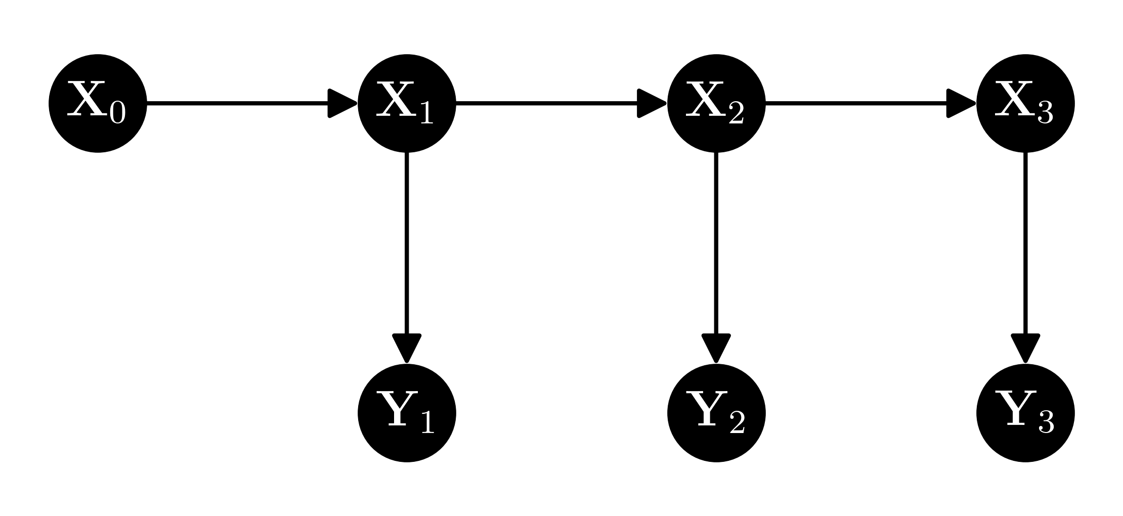
Prove the following statements:

a) $Y_3$ is conditionally independent of $X_1$ given $X_2$.

b) $Y_3$ is conditionally independent of $Y_1$ given $X_2$.

c) $X_3$ is conditionally independent of $X_1$ given $X_2$.

$\lhd$

6.26 Check the calculations in the proof of the Schur Complement Lemma. $\lhd$

6.27 Let $\mathbf{X} = (X_1, X_2, X_3)$ be distributed as $N_3(\bmu, \bSigma)$ where

\[\begin{split} \bmu = \begin{pmatrix} 2\\ -1\\ 3 \end{pmatrix} \qquad \bSigma = \begin{pmatrix} 4 & 1 & 0\\ 1 & 2 & 1\\ 0 & 1 & 3 \end{pmatrix}. \end{split}\]

a) Compute $f_{X_1,X_2|X_3}$, i.e., the conditional density of $(X_1, X_2)$ given $X_3$.

b) What is the correlation coefficient between $X_1$ and $X_2$ under the marginal density $f_{X_1, X_2}$?

$\lhd$

6.28 Consider the block matrix

\[\begin{split} \begin{pmatrix} C & B & \mathbf{0}\\ B^T & \mathbf{0} & D\\ \mathbf{0} & \mathbf{0} & B B^T \end{pmatrix} \end{split}\]

Suppose that $B \in \mathbb{R}^{2 \times 5}$. What are the dimensions of the blocks $C$ and $D$? Justify your answer.

$\lhd$

6.29 a) Let $A_{11} \in \mathbb{R}^{n \times n}$ and $A_{22} \in \mathbb{R}^{m \times m}$ be invertible. Let $A_{12} \in \mathbb{R}^{n \times m}$. Find the inverse of the block matrix

\[\begin{split} A = \begin{pmatrix} A_{11} & A_{12}\\ \mathbf{0} & A_{22} \end{pmatrix}. \end{split}\]

[Hint: You may want to guess what the solution is by considering the case when the blocks are scalars.]

b) Let $\mathbf{b} \in \mathbb{R}^n$ be a non-zero vector. Show that the block matrix

\[\begin{split} B = \begin{pmatrix} I_{n \times n} & \mathbf{b}\\ \mathbf{b}^T & 0 \end{pmatrix} \end{split}\]

is invertible by establishing that $B \mathbf{z} = \mathbf{0}$ implies $\mathbf{z} = \mathbf{0}$. $\lhd$

Exercises

Contents

6.6. Exercises#

6.6.1. Warm-up worksheets#

6.6.2. Problems#