
\(\newcommand{\bmu}{\boldsymbol{\mu}}\) \(\newcommand{\bSigma}{\boldsymbol{\Sigma}}\) \(\newcommand{\bfbeta}{\boldsymbol{\beta}}\) \(\newcommand{\bflambda}{\boldsymbol{\lambda}}\) \(\newcommand{\bgamma}{\boldsymbol{\gamma}}\) \(\newcommand{\bsigma}{{\boldsymbol{\sigma}}}\) \(\newcommand{\bpi}{\boldsymbol{\pi}}\) \(\newcommand{\btheta}{{\boldsymbol{\theta}}}\) \(\newcommand{\bphi}{\boldsymbol{\phi}}\) \(\newcommand{\balpha}{\boldsymbol{\alpha}}\) \(\newcommand{\blambda}{\boldsymbol{\lambda}}\) \(\renewcommand{\P}{\mathbb{P}}\) \(\newcommand{\E}{\mathbb{E}}\) \(\newcommand{\indep}{\perp\!\!\!\perp} \newcommand{\bx}{\mathbf{x}}\) \(\newcommand{\bp}{\mathbf{p}}\) \(\renewcommand{\bx}{\mathbf{x}}\) \(\newcommand{\bX}{\mathbf{X}}\) \(\newcommand{\by}{\mathbf{y}}\) \(\newcommand{\bY}{\mathbf{Y}}\) \(\newcommand{\bz}{\mathbf{z}}\) \(\newcommand{\bZ}{\mathbf{Z}}\) \(\newcommand{\bw}{\mathbf{w}}\) \(\newcommand{\bW}{\mathbf{W}}\) \(\newcommand{\bv}{\mathbf{v}}\) \(\newcommand{\bV}{\mathbf{V}}\) \(\newcommand{\bfg}{\mathbf{g}}\) \(\newcommand{\bfh}{\mathbf{h}}\) \(\newcommand{\horz}{\rule[.5ex]{2.5ex}{0.5pt}}\) \(\renewcommand{\S}{\mathcal{S}}\) \(\newcommand{\X}{\mathcal{X}}\) \(\newcommand{\var}{\mathrm{Var}}\) \(\newcommand{\pa}{\mathrm{pa}}\) \(\newcommand{\Z}{\mathcal{Z}}\) \(\newcommand{\bh}{\mathbf{h}}\) \(\newcommand{\bb}{\mathbf{b}}\) \(\newcommand{\bc}{\mathbf{c}}\) \(\newcommand{\cE}{\mathcal{E}}\) \(\newcommand{\cP}{\mathcal{P}}\) \(\newcommand{\bbeta}{\boldsymbol{\beta}}\) \(\newcommand{\bLambda}{\boldsymbol{\Lambda}}\) \(\newcommand{\cov}{\mathrm{Cov}}\) \(\newcommand{\bfk}{\mathbf{k}}\) \(\newcommand{\idx}[1]{}\) \(\newcommand{\xdi}{}\)
3.6. Application: logistic regression#
We return to logistic regression\(\idx{logistic regression}\xdi\), which we alluded to in the motivating example of this chapter. The input data is of the form \(\{(\boldsymbol{\alpha}_i, b_i) : i=1,\ldots, n\}\) where \(\boldsymbol{\alpha}_i = (\alpha_{i,1}, \ldots, \alpha_{i,d}) \in \mathbb{R}^d\) are the features and \(b_i \in \{0,1\}\) is the label. As before we use a matrix representation: \(A \in \mathbb{R}^{n \times d}\) has rows \(\boldsymbol{\alpha}_i^T\), \(i = 1,\ldots, n\) and \(\mathbf{b} = (b_1, \ldots, b_n) \in \{0,1\}^n\).
3.6.1. Definitions#
We summarize the logistic regression approach. Our goal is to find a function of the features that approximates the probability of the label \(1\). For this purpose, we model the log-odds (or logit function) of the probability of label \(1\) as a linear function of the features \(\boldsymbol{\alpha} \in \mathbb{R}^d\)
where \(\mathbf{x} \in \mathbb{R}^d\) is the vector of coefficients (i.e., parameters). Inverting this expression gives
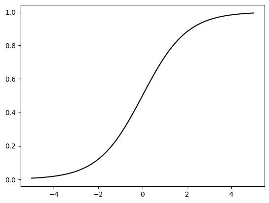
where the sigmoid\(\idx{sigmoid function}\xdi\) function is
for \(z \in \mathbb{R}\).
NUMERICAL CORNER: We plot the sigmoid function.
def sigmoid(z):
    return 1/(1+np.exp(-z))

grid = np.linspace(-5, 5, 100)
plt.plot(grid, sigmoid(grid), c='k')
plt.show()
\(\unlhd\)
We seek to maximize the probability of observing the data (also known as likelihood function) assuming the labels are independent given the features, which is given by (see Chapter 6 for more details; for now we are merely setting up the relevant optimization problem)
Taking a logarithm, multiplying by \(-1/n\) and substituting the sigmoid function, we want to minimize the cross-entropy loss\(\idx{cross-entropy loss}\xdi\)
We used standard properties of the logarithm: for \(x, y > 0\), \(\log(xy) = \log x + \log y\) and \(\log(x^y) = y \log x\).
Hence, we want to solve the minimization problem
We are implicitly using here that the logarithm is a strictly increasing function and therefore does not change the global optimum of a function; multiplying by \(-1/n\) changed the global maximum into a global minimum.
To use gradient descent, we need the gradient of \(\ell\). We use the Chain Rule and first compute the derivative of \(\sigma\) which is
The latter expression is known as the logistic differential equation. It arises in a variety of applications, including the modeling of population dynamics. Here it will be a convenient way to compute the gradient.
Observe that, for \(\boldsymbol{\alpha} = (\alpha_{1}, \ldots, \alpha_{d}) \in \mathbb{R}^d\), by the Chain Rule
where, throughout, the gradient is with respect to \(\mathbf{x}\).
Alternatively, we can obtain the same formula by applying the single-variable Chain Rule
so that
By another application of the Chain Rule, since \(\frac{\mathrm{d}}{\mathrm{d} z} \log z = \frac{1}{z}\),
Using the expression for the gradient of the sigmoid functions, this is equal to
To implement this formula, it will be useful to re-write it in terms of the matrix representation \(A \in \mathbb{R}^{n \times d}\) (which has rows \(\boldsymbol{\alpha}_i^T\), \(i = 1,\ldots, n\)) and \(\mathbf{b} = (b_1, \ldots, b_n) \in \{0,1\}^n\). Let \(\bsigma : \mathbb{R}^n \to \mathbb{R}\) be the vector-valued function that applies the sigmoid \(\sigma\) entry-wise, i.e., \(\bsigma(\mathbf{z}) = (\sigma(z_1),\ldots,\sigma(z_n))\) where \(\mathbf{z} = (z_1,\ldots,z_n)\). Thinking of \(\sum_{i=1}^n (b_i - \sigma(\boldsymbol{\alpha}_i^T \mathbf{x})\,\boldsymbol{\alpha}_i\) as a linear combination of the columns of \(A^T\) with coefficients being the entries of the vector \(\mathbf{b} - \bsigma(A \mathbf{x})\), we that
We turn to the Hessian. By symmetry, we can think of the \(j\)-th column of the Hessian as the gradient of the partial derivative with respect to \(x_j\). Hence we start by computing the gradient of the \(j\)-th entry of the summands in the gradient of \(\ell\). We note that, for \(\boldsymbol{\alpha} = (\alpha_{1}, \ldots, \alpha_{d}) \in \mathbb{R}^d\),
Thus, using the fact that \(\boldsymbol{\alpha} \alpha_{j}\) is the \(j\)-th column of the matrix \(\boldsymbol{\alpha} \boldsymbol{\alpha}^T\), we get
where \(\mathbf{H}_{\ell}(\mathbf{x}; A, \mathbf{b})\) indicates the Hessian with respect to the \(\mathbf{x}\) variables, for fixed \(A, \mathbf{b}\).
LEMMA (Convexity of logistic regression) \(\idx{convexity of logistic regression}\xdi\) The function \(\ell(\mathbf{x}; A, \mathbf{b})\) is convex as a function of \(\mathbf{x} \in \mathbb{R}^d\). \(\flat\)
Proof: Indeed, the Hessian is positive semidefinite: for any \(\mathbf{z} \in \mathbb{R}^d\)
since \(\sigma(t) \in [0,1]\) for all \(t\). \(\square\)
Convexity is one reason for working with the cross-entropy loss (rather than the mean squared error for instance).
LEMMA (Smoothness of logistic regression) The function \(\ell(\mathbf{x}; A, \mathbf{b})\) is \(L\)-smooth for
\(\flat\)
Proof: We use convexity and the expression for the Hessian to derive that, for any unit vector \(\mathbf{z} \in \mathbb{R}^d\),
We need to find the maximum value that the factor \(\sigma(\boldsymbol{\alpha}_i^T \mathbf{x}) (1 - \sigma(\boldsymbol{\alpha}_i^T \mathbf{x}))\) can take. Note that \(\sigma(t) \in [0,1]\) for all \(t\) and \(\sigma(t) + (1 - \sigma(t)) = 1\). Taking the derivatives of the function \(f(w) = w (1 - w) = w - w^2\) we get \(f'(w) = 1 - 2 w\) and \(f''(w) = -2\). So \(f\) is concave and achieve its maximum at \(w^* = 1/2\) where it takes the value \(f(1/2) = 1/4\). We have proved that
for any \(\mathbf{z}\).
Going back to the upper bound on \(\mathbf{z}^T \,\mathbf{H}_{\ell}(\mathbf{x}; A, \mathbf{b}) \,\mathbf{z}\) we get
where we used the Cauchy-Schwarz inequality on the third line and the fact that \(\mathbf{z}\) is a unit vector on the fourth one.
That implies \(L\)-smoothness. \(\square\)
For step size \(\beta\), one step of gradient descent is therefore
3.6.2. Implementation#
We modify our implementation of gradient descent to take a dataset as input. Recall that to run gradient descent, we first implement a function computing a descent update. It takes as input a function grad_fn computing the gradient itself, as well as a current iterate and a step size. We now also feed a dataset as additional input.
def desc_update_for_logreg(grad_fn, A, b, curr_x, beta):
    gradient = grad_fn(curr_x, A, b)
    return curr_x - beta*gradient
We are ready to implement gradient descent. Our function takes as input a function loss_fn computing the objective, a function grad_fn computing the gradient, the dataset A and b, and an initial guess init_x. Optional parameters are the step size and the number of iterations.
def gd_for_logreg(loss_fn, grad_fn, A, b, init_x, beta=1e-3, niters=int(1e5)):
    curr_x = init_x

    for iter in range(niters):
        curr_x = desc_update_for_logreg(grad_fn, A, b, curr_x, beta)

    return curr_x
To implement loss_fn and grad_fn, we define the sigmoid as above. Below, pred_fn is \(\bsigma(A \mathbf{x})\). Here we write the loss function as
where \(\odot\) is the Hadamard product, or element-wise product (for example \(\mathbf{u} \odot \mathbf{v} = (u_1 v_1, \ldots,u_n v_n)\)), the logarithm (denoted in bold) is applied element-wise and \(\mathrm{mean}(\mathbf{z})\) is the mean of the entries of \(\mathbf{z}\) (i.e., \(\mathrm{mean}(\mathbf{z}) = n^{-1} \sum_{i=1}^n z_i\)).
def pred_fn(x, A):
    return sigmoid(A @ x)

def loss_fn(x, A, b):
    return np.mean(-b*np.log(pred_fn(x, A)) - (1 - b)*np.log(1 - pred_fn(x, A)))

def grad_fn(x, A, b):
    return -A.T @ (b - pred_fn(x, A))/len(b)
We can choose a step size based on the smoothness of the objective as above. Recall that numpy.linalg.norm computes the Frobenius norm by default.
def stepsize_for_logreg(A, b):
    L = LA.norm(A)**2 / (4 * len(b))
    return 1/L
NUMERICAL CORNER: We return to our original motivation, the airline customer satisfaction dataset. We first load the dataset. We will need the column names later.
data = pd.read_csv('customer_airline_satisfaction.csv')
column_names = data.columns.tolist()
print(column_names)
['Satisfied', 'Age', 'Class_Business', 'Class_Eco', 'Class_Eco Plus', 'Business travel', 'Loyal customer', 'Flight Distance', 'Departure Delay in Minutes', 'Arrival Delay in Minutes', 'Seat comfort', 'Departure/Arrival time convenient', 'Food and drink', 'Gate location', 'Inflight wifi service', 'Inflight entertainment', 'Online support', 'Ease of Online booking', 'On-board service', 'Leg room service', 'Baggage handling', 'Checkin service', 'Cleanliness', 'Online boarding']
Our goal will be to predict the first column, Satisfied, from the rest of the columns. For this, we transform our data into NumPy arrays. We also standardize the columns by subtracting their mean and dividing by their standard deviation. This will allow to compare the influence of different features on the prediction. And we add a column of 1s to account for the intercept.
y = data['Satisfied'].to_numpy()
X = data.drop(columns=['Satisfied']).to_numpy()

means = np.mean(X, axis=0)
stds = np.std(X, axis=0)
X_standardized = (X - means) / stds

A = np.concatenate((np.ones((len(y),1)), X_standardized), axis=1)
b = y
We use the functions loss_fn and grad_fn which were written for general logistic regression problems.
init_x = np.zeros(A.shape[1])
best_x = gd_for_logreg(loss_fn, grad_fn, A, b, init_x, beta=1e-3, niters=int(1e3))
print(best_x)
[ 0.03622497  0.04123861  0.10020177 -0.08786108 -0.02485893  0.0420605
  0.11995567 -0.01799992 -0.02399636 -0.02653084  0.1176043  -0.02382631
  0.05909378 -0.01161711  0.06553672  0.21313777  0.12883519  0.14631027
  0.12239595  0.11282894  0.08556647  0.08954403  0.08447245  0.108043  ]
To interpret the results, we plot the coefficients in decreasing order.
coefficients, features = best_x[1:], column_names[1:]

sorted_indices = np.argsort(coefficients)
sorted_coefficients = coefficients[sorted_indices]
sorted_features = np.array(features)[sorted_indices]

plt.figure(figsize=(6, 5))
plt.barh(sorted_features, sorted_coefficients, color='lightblue', edgecolor='black')
plt.xlabel('Coefficient Value'), plt.title('Logistic Regression Coefficients')
plt.show()
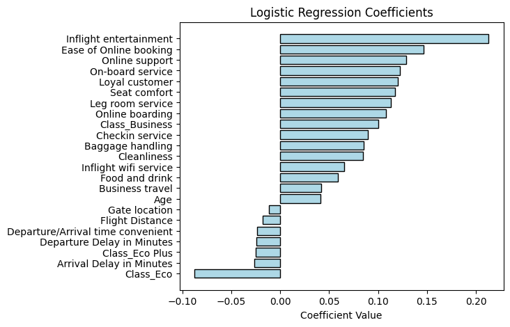
We see from the first ten bars or so that, as might be expected, higher ratings on various aspects of the flight generally contribute to a higher predicted likelihood of satisfaction (with one exception being Gate location whose coefficient is negative but may not be statistically significant). Inflight entertainment seems particularly influential. Age also shows the same pattern, something we had noticed in the introductory section through a different analysis. On the other hand, Departure Delay in Minutes and Arrival Delay in Minutes contribute to a lower predicted likelihood of satisfaction, again an expected pattern. The most negative influence however appears to come from Class_Eco.
CHAT & LEARN There are faster methods for logistic regression. Ask your favorite AI chatbot for an explanation and implementation of the iteratively reweighted least squares method. Try it on this dataset. (Open In Colab) \(\ddagger\)
TRY IT! One can attempt to predict whether a new customer, whose feature vector is \(\boldsymbol{\alpha}\), will be satisfied by using the prediction function \(p(\mathbf{x}; \boldsymbol{\alpha}) = \sigma(\boldsymbol{\alpha}^T \mathbf{x})\), where \(\mathbf{x}\) is the fitted coefficients. Say a customer is predicted to be satisfied if \(\sigma(\boldsymbol{\alpha}^T \mathbf{x}) > 0.5\). Implement this predictor and compute its accuracy on this dataset. (Open In Colab)
CHAT & LEARN Because of the issue of overfitting, computing the accuracy of a predictor on a dataset used to estimate the coefficients is problematic. Ask your favorite AI chatbot about scikit-learn’s train_test_split function and how it helps resolve this issue. Implement it on this dataset. (Open In Colab) \(\ddagger\)
\(\unlhd\)
Self-assessment quiz (with help from Claude, Gemini, and ChatGPT)
1 What is the primary goal of logistic regression?
a) To predict a continuous outcome variable.
b) To classify data points into multiple categories.
c) To model the probability of a binary outcome.
d) To find the optimal linear combination of features.
2 What is the relationship between maximizing the likelihood function and minimizing the cross-entropy loss in logistic regression?
a) They are unrelated concepts.
b) Maximizing the likelihood is equivalent to minimizing the cross-entropy loss.
c) Minimizing the cross-entropy loss is a first step towards maximizing the likelihood.
d) Maximizing the likelihood is a special case of minimizing the cross-entropy loss.
3 Which of the following is the correct formula for the logistic regression objective function (cross-entropy loss)?
a) \(\ell(\mathbf{x}; A, \mathbf{b}) = \frac{1}{n} \sum_{i=1}^n \log(1 + \exp(-b_i \boldsymbol{\alpha}_i^T \mathbf{x}))\)
b) \(\ell(\mathbf{x}; A, \mathbf{b}) = \frac{1}{n} \sum_{i=1}^n (b_i - \sigma(\boldsymbol{\alpha}_i^T \mathbf{x}))^2\)
c) \(\ell(\mathbf{x}; A, \mathbf{b}) = \frac{1}{n} \sum_{i=1}^n \{-b_i \log(\sigma(\boldsymbol{\alpha}_i^T \mathbf{x})) - (1 - b_i) \log(1 - \sigma(\boldsymbol{\alpha}_i^T \mathbf{x}))\}\)
d) \(\ell(\mathbf{x}; A, \mathbf{b}) = \frac{1}{n} \sum_{i=1}^n b_i \boldsymbol{\alpha}_i^T \mathbf{x}\)
4 What is the purpose of standardizing the input features in the airline customer satisfaction dataset example?
a) To ensure the objective function is convex.
b) To speed up the convergence of gradient descent.
c) To allow comparison of the influence of different features on the prediction.
d) To handle missing data in the dataset.
5 Which of the following is a valid reason for adding a column of 1’s to the feature matrix in logistic regression?
a) To ensure the objective function is convex.
b) To allow for an intercept term in the model.
c) To standardize the input features.
d) To handle missing data in the dataset.
Answer for 1: c. Justification: The text states that the goal of logistic regression is to “find a function of the features that approximates the probability of the label.”
Answer for 2: b. Justification: The text states: “We seek to maximize the probability of observing the data… which is given by… Taking a logarithm, multiplying by \(-1/n\) and substituting the sigmoid function, we want to minimize the cross-entropy loss.”
Answer for 3: c. Justification: The text states: “Hence, we want to solve the minimization problem \(\min_{x \in \mathbb{R}^d} \ell(\mathbf{x}; A, \mathbf{b})\),” where \(\ell(\mathbf{x}; A, \mathbf{b}) = \frac{1}{n} \sum_{i=1}^n \{-b_i \log(\sigma(\boldsymbol{\alpha}_i^T \mathbf{x})) - (1 - b_i) \log(1 - \sigma(\boldsymbol{\alpha}_i^T \mathbf{x}))\}\).
Answer for 4: c. Justification: The text states: “We also standardize the columns by subtracting their mean and dividing by their standard deviation. This will allow to compare the influence of different features on the prediction.”
Answer for 5: b. Justification: The text states: “To allow an affine function of the features, we add a column of 1’s as we have done before.”