\(\newcommand{\bSigma}{\boldsymbol{\Sigma}}\) \(\newcommand{\bmu}{\boldsymbol{\mu}}\)

5.8. Online supplementary material

5.8.1. Quizzes, solutions, code, etc.

5.8.1.1. Just the code

An interactive Jupyter notebook featuring the code in this chapter can be accessed below (Google Colab recommended). You are encouraged to tinker with it. Some suggested computational exercises are scattered throughout. The notebook is also available as a slideshow.

• Notebook (Open In Colab)

• Slideshow

5.8.1.2. Self-assessment quizzes

A more extensive web version of the self-assessment quizzes is available by following the links below.

• Section 5.2

• Section 5.3

• Section 5.4

• Section 5.5

• Section 5.6

5.8.1.3. Auto-quizzes

Automatically generated quizzes for this chapter can be accessed here (Google Colab recommended).

• Auto-quizzes (Open In Colab)

5.8.1.4. Solutions to odd-numbered warm-up exercises

(with help from Claude, Gemini, and ChatGPT)

E5.2.1 \(V = \{1, 2, 3, 4\}\), \(E = \{\{1, 2\}, \{1, 3\}, \{2, 4\}, \{3, 4\}\}\). This follows directly from the definition of a graph as a pair \(G = (V, E)\).

E5.2.3 One possible path is \(1 \sim 2 \sim 4\). Its length is 2, since it consists of two edges.

E5.2.5 \(\delta^-(2) = 1\), \(\delta^+(2) = 2\). The in-degree of a vertex \(v\) is the number of edges with destination \(v\), and the out-degree is the number of edges with source \(v\).

E5.2.7 The graph \(G\) is not connected. There is no path between vertex 1 and vertex 4, indicating that the graph is not connected.

E5.2.9 The number of connected components is 1. There is a path between every pair of vertices, so the graph is connected, having only one connected component.

E5.2.11

\[\begin{split} B = \begin{pmatrix} 1 & 1 & 0 & 0 \\ 1 & 0 & 1 & 0 \\ 0 & 1 & 0 & 1 \\ 0 & 0 & 1 & 1 \end{pmatrix}. \end{split}\]

The entry \(B_{ij}\) is 1 if vertex \(i\) is incident to edge \(j\), and 0 otherwise.

E5.2.13

\[\begin{split} B = \begin{pmatrix} -1 & 0 & 1 & 0 \\ 1 & -1 & 0 & -1 \\ 0 & 1 & -1 & 0 \\ 0 & 0 & 0 & 1 \end{pmatrix}. \end{split}\]

The entry \(B_{ij}\) is 1 if edge \(j\) leaves vertex \(i\), -1 if edge \(j\) enters vertex \(i\), and 0 otherwise.

E5.2.15 The Petersen graph is 3-regular, as stated in the text.

E5.3.1 We can find the eigenvectors of \(A\) and normalize them to get an orthonormal basis. The characteristic polynomial of \(A\) is \((5-\lambda)^2 - 9 = \lambda^2 - 10\lambda + 16 = (\lambda - 2)(\lambda - 8)\), so the eigenvalues are 2 and 8. For \(\lambda = 2\), an eigenvector is \(\begin{pmatrix} -1 \\ 1 \end{pmatrix}\), and for \(\lambda = 8\), an eigenvector is \(\begin{pmatrix} 1 \\ 1 \end{pmatrix}\). Normalizing these vectors, we get the matrix

\[\begin{split} W = \begin{pmatrix} -1/\sqrt{2} & 1/\sqrt{2} \\ 1/\sqrt{2} & 1/\sqrt{2} \end{pmatrix}. \end{split}\]

E5.3.3 \(R_A(u) = \frac{\langle u, Au \rangle}{\langle u, u \rangle} = \langle u, Au \rangle = \begin{pmatrix} \frac{\sqrt{3}}{2} & \frac{1}{2} \end{pmatrix} \begin{pmatrix} 3 & 1 \\ 1 & 2 \end{pmatrix} \begin{pmatrix} \frac{\sqrt{3}}{2} \\ \frac{1}{2} \end{pmatrix} = \frac{7}{2}\).

E5.3.5 To find the eigenvalues, we solve the characteristic equation: \(\det(A - \lambda I) = \begin{vmatrix} 2-\lambda & -1 \\ -1 & 2-\lambda \end{vmatrix} = (2-\lambda)^2 - 1 = \lambda^2 - 4\lambda + 3 = (\lambda - 1)(\lambda - 3) = 0\). So the eigenvalues are \(\lambda_1 = 3\) and \(\lambda_2 = 1\). To find the eigenvectors, we solve \((A - \lambda_i I)v_i = 0\) for each eigenvalue: For \(\lambda_1 = 3\): \(\begin{pmatrix} -1 & -1 \\ -1 & -1 \end{pmatrix}v_1 = 0\), which gives \(v_1 = c\begin{pmatrix} 1 \\ -1 \end{pmatrix}\). Normalizing, we get \(v_1 = \frac{1}{\sqrt{2}}\begin{pmatrix} 1 \\ -1 \end{pmatrix}\). For \(\lambda_2 = 1\): \(\begin{pmatrix} 1 & -1 \\ -1 & 1 \end{pmatrix}v_2 = 0\), which gives \(v_2 = c\begin{pmatrix} 1 \\ 1 \end{pmatrix}\). Normalizing, we get \(v_2 = \frac{1}{\sqrt{2}}\begin{pmatrix} 1 \\ 1 \end{pmatrix}\). To verify the variational characterization for \(\lambda_1\): \(R_A(v_1) = \frac{\langle v_1, Av_1 \rangle}{\langle v_1, v_1 \rangle} = \frac{1}{2}\begin{pmatrix} 1 & 1 \end{pmatrix}\begin{pmatrix} 2 & -1 \\ -1 & 2 \end{pmatrix}\begin{pmatrix} 1 \\ 1 \end{pmatrix} = \frac{1}{2}(2 - 1 - 1 + 2) = 3 = \lambda_1\). For any unit vector \(u = \begin{pmatrix} \cos\theta \\ \sin\theta \end{pmatrix}\), we have: \(R_A(u) = \begin{pmatrix} \cos\theta & \sin\theta \end{pmatrix}\begin{pmatrix} 2 & -1 \\ -1 & 2 \end{pmatrix}\begin{pmatrix} \cos\theta \\ \sin\theta \end{pmatrix} = 2\cos^2\theta + 2\sin^2\theta - 2\cos\theta\sin\theta = 2 - 2\cos\theta\sin\theta \leq 2 + 2|\cos\theta\sin\theta| \leq 3\), with equality when \(\theta = \frac{\pi}{4}\), which corresponds to \(u = v_1\). Thus, \(\lambda_1 = \max_{u \neq 0} R_A(u)\).

E5.3.7 First, we find the eigenvalues corresponding to the given eigenvectors: \(Av_1 = \begin{pmatrix} 1 & 2 & 0 \\ 2 & 1 & 0 \\ 0 & 0 & 3 \end{pmatrix} \frac{1}{\sqrt{2}} \begin{pmatrix} 1 \\ 1 \\ 0 \end{pmatrix} = \frac{1}{\sqrt{2}} \begin{pmatrix} 3 \\ 3 \\ 0 \end{pmatrix} = 3v_1\), so \(\lambda_1 = 3\). \(Av_2 = \begin{pmatrix} 1 & 2 & 0 \\ 2 & 1 & 0 \\ 0 & 0 & 3 \end{pmatrix} \frac{1}{\sqrt{2}} \begin{pmatrix} -1 \\ 1 \\ 0 \end{pmatrix} = \frac{1}{\sqrt{2}} \begin{pmatrix} -1 \\ 1 \\ 0 \end{pmatrix} = v_2\), so \(\lambda_2 = 1\). \(Av_3 = \begin{pmatrix} 1 & 2 & 0 \\ 2 & 1 & 0 \\ 0 & 0 & 3 \end{pmatrix} \begin{pmatrix} 0 \\ 0 \\ 1 \end{pmatrix} = \begin{pmatrix} 0 \\ 0 \\ 3 \end{pmatrix} = 3v_3\), so \(\lambda_3 = 3\).

So the eigenvalues are \(\lambda_1 = 3\), \(\lambda_2 = 1\), and \(\lambda_3 = 3\). Note that \(\lambda_2\) is the second smallest eigenvalue.

Now, let’s verify the variational characterization for \(\lambda_2\). Any vector \(u \in V_2\) can be written as \(u = c_1 v_1 + c_2 v_2\) for some scalars \(c_1\) and \(c_2\). Then:

\(\langle u, u \rangle = \langle c_1 v_1 + c_2 v_2, c_1 v_1 + c_2 v_2 \rangle = c_1^2 \langle v_1, v_1 \rangle + 2c_1c_2 \langle v_1, v_2 \rangle + c_2^2 \langle v_2, v_2 \rangle = c_1^2 + c_2^2\), since \(v_1\) and \(v_2\) are orthonormal.

\(\langle u, Au \rangle = \langle c_1 v_1 + c_2 v_2, A(c_1 v_1 + c_2 v_2) \rangle = \langle c_1 v_1 + c_2 v_2, 3c_1 v_1 + c_2 v_2 \rangle = 3c_1^2 + c_2^2\), since \(Av_1 = 3v_1\) and \(Av_2 = v_2\).

Therefore, \(R_A(u) = \frac{\langle u, Au \rangle}{\langle u, u \rangle} = \frac{3c_1^2 + c_2^2}{c_1^2 + c_2^2} \geq 1\) for all \(u \neq 0\) in \(V_2\), with equality when \(c_1 = 0\). Thus: \(\lambda_2 = \min_{0 \neq u \in V_2} R_A(u) = 1 = R_A(v_2)\).

So indeed, the second smallest eigenvalue \(\lambda_2\) satisfies the variational characterization \(\lambda_2 = \min_{0 \neq u \in V_2} R_A(u)\).

E5.4.1 The degree matrix \(D\) is

\[\begin{split} D = \begin{pmatrix} 1 & 0 & 0 & 0 \\ 0 & 3 & 0 & 0 \\ 0 & 0 & 2 & 0 \\ 0 & 0 & 0 & 2 \end{pmatrix}. \end{split}\]

The Laplacian matrix \(L\) is \(L = D - A\):

\[\begin{split} L = \begin{pmatrix} 1 & -1 & 0 & 0 \\ -1 & 3 & -1 & -1 \\ 0 & -1 & 2 & -1 \\ 0 & -1 & -1 & 2 \end{pmatrix}. \end{split}\]

E5.4.3

\[\begin{split} Ly_1 = \begin{pmatrix} 2 & -1 & 0 & -1 & 0\\ -1 & 2 & -1 & 0 & 0\\ 0 & -1 & 3 & -1 & -1\\ -1 & 0 & -1 & 2 & 0\\ 0 & 0 & -1 & 0 & 1 \end{pmatrix} \cdot \frac{1}{\sqrt{5}}\begin{pmatrix} 1\\ 1\\ 1\\ 1\\ 1 \end{pmatrix} = \frac{1}{\sqrt{5}}\begin{pmatrix} 0\\ 0\\ 0\\ 0\\ 0 \end{pmatrix} = 0 \cdot y_1. \end{split}\]

E5.4.5 Let’s verify that \(y_1\) and \(y_2\) are eigenvectors of \(L\):

\[\begin{split} Ly_1 = \begin{pmatrix} 1 & -1 & 0 & 0\\ -1 & 2 & -1 & 0\\ 0 & -1 & 2 & -1\\ 0 & 0 & -1 & 1 \end{pmatrix} \cdot \frac{1}{2}\begin{pmatrix} 1\\ 1\\ 1\\ 1 \end{pmatrix} = \frac{1}{2}\begin{pmatrix} 0\\ 0\\ 0\\ 0 \end{pmatrix} = 0 \cdot y_1, \end{split}\]

\[\begin{split} Ly_2 = \begin{pmatrix} 1 & -1 & 0 & 0\\ -1 & 2 & -1 & 0\\ 0 & -1 & 2 & -1\\ 0 & 0 & -1 & 1 \end{pmatrix} \cdot \frac{1}{2}\begin{pmatrix} 1\\ \frac{1}{\sqrt{2}}\\ -\frac{1}{\sqrt{2}}\\ -1 \end{pmatrix} = (2 - \sqrt{2}) \cdot \frac{1}{2}\begin{pmatrix} 1\\ \frac{1}{\sqrt{2}}\\ -\frac{1}{\sqrt{2}}\\ -1 \end{pmatrix} = (2 - \sqrt{2}) \cdot y_2. \end{split}\]

So, \(y_1\) is an eigenvector with eigenvalue \(\mu_1 = 0\), and \(y_2\) is an eigenvector with eigenvalue \(\mu_2 = 2 - \sqrt{2}\).

E5.4.7 The maximum degree of \(K_4\) is \(\bar{\delta} = 3\). Using the bounds \(\bar{\delta} + 1 \leq \mu_n \leq 2\bar{\delta}\), we have:

\[ 4 = \bar{\delta} + 1 \leq \mu_4 \leq 2\bar{\delta} = 6. \]

E5.4.9 The diagonal entry \(L_{ii}\) is the degree of vertex \(i\), and the off-diagonal entry \(L_{ij}\) (for \(i \neq j\)) is \(-1\) if vertices \(i\) and \(j\) are adjacent, and 0 otherwise. Thus, the sum of the entries in row \(i\) is

\[ \deg(i) - \sum_{j: \{i,j\} \in E} 1 = 0. \]

E5.4.11 For any vector \(x \in \mathbb{R}^n\), we have

\[ x^T L_G x = \sum_{\{i,j\} \in E} (x_i - x_j)^2 \ge 0. \]

Since this holds for all \(x\), \(L_G\) is positive semidefinite.

E5.4.13 In a complete graph, each vertex has degree \(n-1\). Thus, the Laplacian matrix is \(L_G = nI - J\), where \(I\) is the identity matrix and \(J\) is the all-ones matrix. The eigenvalues of \(J\) are \(n\) (with multiplicity 1) and, because \(J\) has rank one, 0 (with multiplicity \(n-1\)). Therefore, the eigenvalues of \(L_G\) are 0 (with multiplicity 1) and \(n\) (with multiplicity \(n-1\)).

E5.5.1 \(|E(S, S^c)| = 2\) (the edges between \(S\) and \(S^c\) are \(\{1, 2\}\) and \(\{2, 3\}\)), and \(\min\{|S|, |S^c|\} = 1\). Therefore, \(\phi(S) = \frac{|E(S, S^c)|}{\min\{|S|, |S^c|\}} = 2\).

E5.5.3 In a connected graph with \(n\) vertices, the numerator of the cut ratio is at least 1, and the denominator is at most \(n/2\), which is achieved by cutting the graph into two equal parts. Therefore, the smallest possible value of the isoperimetric number is \(\frac{1}{n/2} = \frac{2}{n}\). For \(n = 6\), this is \(\frac{1}{3}\).

E5.5.5 The Cheeger Inequality also states that \(\frac{\phi_G^2}{2\bar{\delta}} \leq \mu_2\). Therefore, \(\phi_G \leq \sqrt{2\bar{\delta}\mu_2} = \sqrt{2 \cdot 4 \cdot 0.5} = 2\).

E5.5.7 Let \(\mathbf{v}_1 = (1, 1, 1, 1)/2\), \(\mathbf{v}_2 = (-1, -1, 1, 1)/2\), \(\mathbf{v}_3 = (1, -1, -1, 1)/2\), and \(\mathbf{v}_4 = (1, -1, 1, -1)/2\). These vectors form an orthonormal list. We can verify that these are eigenvectors of \(L\) and find their corresponding eigenvalues:

\[\begin{split} L\mathbf{v}_1 = \begin{pmatrix} 2 & -1 & 0 & -1 \\ -1 & 2 & -1 & 0 \\ 0 & -1 & 2 & -1 \\ -1 & 0 & -1 & 2 \end{pmatrix} \frac{1}{2}\begin{pmatrix} 1 \\ 1 \\ 1 \\ 1 \end{pmatrix} = \begin{pmatrix} 0 \\ 0 \\ 0 \\ 0 \end{pmatrix} = 0 \cdot \mathbf{v}_1, \end{split}\]

\[\begin{split} L\mathbf{v}_2 = \begin{pmatrix} 2 & -1 & 0 & -1 \\ -1 & 2 & -1 & 0 \\ 0 & -1 & 2 & -1 \\ -1 & 0 & -1 & 2 \end{pmatrix} \frac{1}{2}\begin{pmatrix} -1 \\ -1 \\ 1 \\ 1 \end{pmatrix} = \frac{1}{2}\begin{pmatrix} -2 \\ -2 \\ 2 \\ 2 \end{pmatrix} = 2 \cdot \mathbf{v}_2, \end{split}\]

\[\begin{split} L\mathbf{v}_3 = \begin{pmatrix} 2 & -1 & 0 & -1 \\ -1 & 2 & -1 & 0 \\ 0 & -1 & 2 & -1 \\ -1 & 0 & -1 & 2 \end{pmatrix} \frac{1}{2}\begin{pmatrix} 1 \\ -1 \\ -1 \\ 1 \end{pmatrix} = \frac{1}{2}\begin{pmatrix} 2 \\ -2 \\ -2 \\ 2 \end{pmatrix} = 2 \cdot \mathbf{v}_3, \end{split}\]

\[\begin{split} L\mathbf{v}_4 = \begin{pmatrix} 2 & -1 & 0 & -1 \\ -1 & 2 & -1 & 0 \\ 0 & -1 & 2 & -1 \\ -1 & 0 & -1 & 2 \end{pmatrix} \frac{1}{2}\begin{pmatrix} 1 \\ -1 \\ 1 \\ -1 \end{pmatrix} = \frac{1}{2}\begin{pmatrix} 4 \\ -4 \\ 4 \\ -4 \end{pmatrix} = 4 \cdot \mathbf{v}_4. \end{split}\]

Therefore, the corresponding eigenvalues are \(\mu_1 = 0\), \(\mu_2 = 2\), \(\mu_3 = 2\), and \(\mu_4 = 4\).

E5.5.9 Using the Fiedler vector \(\mathbf{v}_2 = (-1, -1, 1, 1)/2\), an order is \(\pi(1) = 1\), \(\pi(2) = 2\), \(\pi(3) = 3\), \(\pi(4) = 4\).

E5.5.11 To find the isoperimetric number, we need to consider all possible cuts and find the minimum cut ratio.

Let’s consider all possible cuts:

• \(S = \{1\}\), \(|E(S, S^c)| = 2\), \(\min\{|S|, |S^c|\} = 1\), so \(\phi(S) = 2\).

• \(S = \{1, 2\}\), \(|E(S, S^c)| = 2\), \(\min\{|S|, |S^c|\} = 2\), so \(\phi(S) = 1\).

• \(S = \{1, 2, 3\}\), \(|E(S, S^c)| = 2\), \(\min\{|S|, |S^c|\} = 1\), so \(\phi(S) = 2\).

• \(S = \{1, 2, 3, 4\}\), \(|E(S, S^c)| = 2\), \(\min\{|S|, |S^c|\} = 0\), so \(\phi(S)\) is undefined.

• etc.

The minimum cut ratio is \(1\), achieved by the cut \(S = \{1, 2\}\). Therefore, the isoperimetric number of the graph is \(\phi_G = 1\).

Comparing this to the results from E5.5.8 and E5.5.10:

• In E5.5.8, we found that the Fiedler vector is either \((-1, -1, 1, 1)/2\), which suggests a cut separating vertices \(\{1, 2\}\) from \(\{3, 4\}\).

• In E5.5.10, using the ordering based on the Fiedler vector, we found that the cut with the smallest ratio is \(S_2 = \{1, 2\}\), with a cut ratio of \(1\).

Both the Fiedler vector and the spectral clustering algorithm based on it correctly identify the cut that achieves the isoperimetric number (Cheeger constant) of the graph.

Now, let’s compare the isoperimetric number to the bounds given by Cheeger’s inequality. From E5.5.7, we know that the second smallest eigenvalue of the Laplacian matrix is \(\mu_2 = 2\). The maximum degree of the graph is \(\bar{\delta} = 2\). Cheeger’s inequality states that:

\[\frac{\phi_G^2}{2\bar{\delta}} \leq \mu_2 \leq 2\phi_G\]

Plugging in the values, we get:

\[\frac{(\frac{1}{2})^2}{2 \cdot 2} \leq 2 \leq 2 \cdot 1\]

which simplifies to:

\[\frac{1}{16} \leq 2 \leq 2\]

We can see that the isoperimetric number \(\phi_G = 1\) satisfies the bounds given by Cheeger’s inequality.

E5.5.13

\[\begin{split} D = \begin{pmatrix} 2 & 0 & 0 & 0 & 0 \\ 0 & 3 & 0 & 0 & 0 \\ 0 & 0 & 3 & 0 & 0 \\ 0 & 0 & 0 & 1 & 0 \\ 0 & 0 & 0 & 0 & 1 \\ \end{pmatrix} \end{split}\]

The degree matrix \(D\) is a diagonal matrix where each entry \(D_{ii}\) is the degree of vertex \(i\).

E5.5.15

\[ \text{Cutset} = \{\{1, 3\}, \{2, 3\}, \{2, 4\}\}, \quad |E(S, S^c)| = 3 \]

\[ \phi(S) = \frac{|E(S, S^c)|}{\min(|S|, |S^c|)} = \frac{3}{2} = 1.5 \]

The cutset consists of edges between \(S\) and \(S^c\). The cut ratio \(\phi(S)\) is the

size of the cutset divided by the size of the smaller subset.

E5.5.17

import networkx as nx
import matplotlib.pyplot as plt

G = nx.Graph()
edges = [(1, 2), (1, 3), (2, 3), (2, 4), (3, 5)]
G.add_edges_from(edges)
pos = nx.spring_layout(G)

nx.draw(G, pos, with_labels=True, node_color='lightblue', node_size=500, font_size=15)
nx.draw_networkx_edges(G, pos, edgelist=[(1, 3), (2, 3), (2, 4)], edge_color='r', width=2)
plt.show()

This code creates and displays the graph with the cut edges highlighted in red.

E5.6.1 The expected number of edges is \(\mathbb{E}[|E|] = \binom{n}{2}p = \binom{6}{2} \cdot 0.4 = 15 \cdot 0.4 = 6\).

E5.6.3 The expected number of triangles is \(\mathbb{E}[|T_3|] = \binom{n}{3}p^3 = \binom{10}{3} \cdot 0.3^3 = 120 \cdot 0.027 = 3.24\). The expected triangle density is \(\mathbb{E}[|T_3|/\binom{n}{3}] = p^3 = 0.3^3 = 0.027\).

E5.6.5 The block assignment matrix \(Z\) is given by:

\[\begin{split} Z = \begin{pmatrix} 1 & 0 \\ 1 & 0 \\ 1 & 0 \\ 1 & 0 \\ 0 & 1 \\ 0 & 1 \\ 0 & 1 \\ 0 & 1 \end{pmatrix}. \end{split}\]

E5.6.7 The degree of a vertex in \(G(4, 0.5)\) follows a binomial distribution \(\mathrm{Bin}(3, 0.5)\). The probabilities are:

• \(\mathbb{P}(d = 0) = (0.5)^3 = 0.125\)

• \(\mathbb{P}(d = 1) = 3 \cdot (0.5)^3 = 0.375\)

• \(\mathbb{P}(d = 2) = 3 \cdot (0.5)^3 = 0.375\)

• \(\mathbb{P}(d = 3) = (0.5)^3 = 0.125\)

E5.6.9 The variance is \(\mathrm{Var}[|E|] = \binom{3}{2} \cdot p \cdot (1 - p) = 3 \cdot 0.5 \cdot 0.5 = 0.75\).

E5.6.11 Since vertex 2 is in block \(C_1\) and vertex 4 is in block \(C_2\), the probability of an edge between them is \(b_{1,2} = 1/4\).

E5.6.13 The expected degree of each vertex is \((p+q)n/2 = (1)(8)/2 = 4\).

E5.6.15 Let \(A_{i,j}\) be the indicator random variable for the presence of edge \(\{i,j\}\). Then the number of edges is \(X = \sum_{i<j} A_{i,j}\). Since the edges are independent,

\[\begin{align*} \mathrm{Var}[X] &= \mathrm{Var}\left[\sum_{i<j} A_{i,j}\right] \\ &= \sum_{i<j} \mathrm{Var}[A_{i,j}] \\ &= \sum_{i<j} m_{i,j}(1-m_{i,j}) \\ &= \frac{1}{2}\left(1-\frac{1}{2}\right) + \frac{1}{4}\left(1-\frac{1}{4}\right) + \frac{1}{2}\left(1-\frac{1}{2}\right) \\ &= \frac{11}{16}. \end{align*}\]

5.8.1.5. Learning outcomes

• Define undirected and directed graphs, and identify their key components such as vertices, edges, paths, and cycles.

• Recognize special types of graphs, including cliques, trees, forests, and directed acyclic graphs (DAGs).

• Determine the connectivity of a graph and identify its connected components.

• Construct the adjacency matrix, incidence matrix, and Laplacian matrix representations of a graph.

• Prove key properties of the Laplacian matrix, such as symmetry and positive semidefiniteness.

• Extend the concepts of graphs and their matrix representations to weighted graphs.

• Implement graph representations and algorithms using the NetworkX package in Python.

• Apply graph theory concepts to model and analyze real-world networks and relationships.

• Outline the proof of the Spectral Theorem using a sequence of orthogonal transformations to diagonalize a matrix.

• Define the Rayleigh quotient and explain its relationship to eigenvectors and eigenvalues.

• Prove the variational characterizations of the largest, smallest, and second smallest eigenvalues of a symmetric matrix using the Rayleigh quotient.

• State the Courant-Fischer Theorem and interpret its local and global formulas for the eigenvalues of a symmetric matrix.

• Apply the Courant-Fischer Theorem to characterize the third smallest eigenvalue of a symmetric matrix.

• State the key properties of the Laplacian matrix, including symmetry, positive semidefiniteness, and the constant eigenvector associated with the zero eigenvalue.

• Prove the relationship between graph connectivity and the second smallest eigenvalue (algebraic connectivity) of the Laplacian matrix.

• Derive bounds on the largest eigenvalue of the Laplacian matrix using the maximum degree of the graph.

• Formulate the variational characterization of the second smallest eigenvalue of the Laplacian matrix as a constrained optimization problem.

• Explain how the eigenvectors of the Laplacian matrix can be used for graph drawing and revealing the underlying geometry of the graph, using the variational characterization.

• Compute the Laplacian matrix and its eigenvalues and eigenvectors for simple graphs, and interpret the results in terms of graph connectivity and geometry.

• Compute the cut ratio and the isoperimetric number (Cheeger constant) for a given graph cut.

• State the Cheeger Inequality and explain its significance in relating the isoperimetric number to the second smallest Laplacian eigenvalue.

• Describe the main steps of the graph-cutting algorithm based on the Fiedler vector.

• Analyze the performance guarantees of the Fiedler vector-based graph-cutting algorithm and compare them to the optimal cut.

• Apply spectral clustering techniques to identify communities within a graph, and evaluate the quality of the resulting partitions.

• Formulate the minimum bisection problem as a discrete optimization problem and relax it into a continuous optimization problem related to the Laplacian matrix.

• Define the inhomogeneous Erdős-Rényi (ER) random graph model and explain how it generalizes the standard ER model.

• Generate inhomogeneous ER graphs and analyze their properties, such as edge density and the probability of connectivity, using Python and NetworkX.

• Calculate the expected number of edges and triangles in an ER random graph.

• Describe the stochastic blockmodel (SBM) and its role in creating random graphs with planted partitions, and explain how it relates to the concept of homophily.

• Construct SBMs with specified block assignments and edge probabilities, and visualize the resulting graphs using Python and NetworkX.

• Compute the expected adjacency matrix of an SBM given the block assignment matrix and connection probabilities.

• Apply spectral clustering algorithms to SBMs and evaluate their performance in recovering the ground truth community structure.

• Analyze the simplified symmetric stochastic blockmodel (SSBM) and derive the spectral decomposition of its expected adjacency matrix.

• Explain the relationship between the eigenvectors of the expected Laplacian matrix and the community structure in the SSBM.

• Investigate the behavior of the eigenvalues of the Laplacian matrix for large random graphs and discuss the connection to random matrix theory.

\(\aleph\)

5.8.2. Additional sections

5.8.2.1. Spectral properties of SBM

The SBM provides an alternative explanation for the efficacy of spectral clustering.

We use a toy version of the model. Specifically, we assume that:

• The number of vertices \(n\) is even.

• Vertices \(1,\ldots,n/2\) are in block \(C_1\) while vertices \(n/2+1,\ldots,n\) are in block \(C_2\).

• The intra-block connection probability is \(b_{1,1} = b_{2,2} = p\) and the inter-block connection probability is \(b_{1,2} = b_{2,1} = q < p\), with \(p, q \in (0,1)\).

• We allow self-loops, whose probability are the intra-block connection probability.

In that case, the matrix \(M\) is the block matrix

\[\begin{split} M = \begin{pmatrix} p J & q J\\ qJ & pJ \end{pmatrix}, \end{split}\]

where \(J \in \mathbb{R}^{n/2 \times n/2}\) is the all-one matrix. We refer to this model as the symmetric stochastic blockmodel (SSBM).

The matrix \(M\) is symmetric. Hence it has a spectral decomposition. It is straightforward to compute. Let \(\mathbf{1}_m\) be the all-one vector of size \(m\).

LEMMA (Spectral Decomposition of SSBM) Consider the matrix \(M\) above. Let

\[\begin{split} \mathbf{q}_1 = \frac{1}{\sqrt{n}} \mathbf{1}_n \quad \text{and} \quad \mathbf{q}_2 = \frac{1}{\sqrt{n}} \begin{pmatrix} \mathbf{1}_{n/2} \\ - \mathbf{1}_{n/2} \end{pmatrix}. \end{split}\]

Let \(\mathbf{q}_3,\ldots,\mathbf{q}_n\) be an orthonormal basis of \((\mathrm{span}\{\mathbf{q}_1, \mathbf{q}_2\})^\perp\). Denote by \(Q\) the matrix whose columns are \(\mathbf{q}_1,\ldots,\mathbf{q}_n\). Let

\[ \lambda_1 = \frac{p + q}{2} n \quad \text{and} \quad \lambda_2 = \frac{p - q}{2} n. \]

Let \(\lambda_3,\ldots,\lambda_n = 0\). Denote by \(\Lambda\) the diagonal matrix with diagonal entries \(\lambda_1,\ldots,\lambda_n\).

Then a spectral decomposition of \(M\) is given by

\[ M = Q \Lambda Q^T. \]

In particular, \(\mathbf{q}_i\) is an eigenvector of \(M\) with eigenvalue \(\lambda_i\). \(\flat\)

Proof: We start with \(\mathbf{q}_1\) and note that by the formula for the multiplication of block matrices and the definition of \(J\)

\[\begin{align*} M \mathbf{q}_1 &= \begin{pmatrix} p J & q J\\ q J & p J \end{pmatrix} \frac{1}{\sqrt{n}} \mathbf{1}_n \\ &= \begin{pmatrix} p J & q J\\ q J & p J \end{pmatrix} \frac{1}{\sqrt{n}} \begin{pmatrix} \mathbf{1}_{\frac{n}{2}} \\ \mathbf{1}_{\frac{n}{2}} \end{pmatrix} \\ &= \frac{1}{\sqrt{n}} \begin{pmatrix} p J \mathbf{1}_{\frac{n}{2}} + q J \mathbf{1}_{\frac{n}{2}}\\ q J \mathbf{1}_{\frac{n}{2}} + p J \mathbf{1}_{\frac{n}{2}} \end{pmatrix} \\ &= \frac{1}{\sqrt{n}} \begin{pmatrix} (p + q) J \mathbf{1}_{\frac{n}{2}}\\ (p + q) J \mathbf{1}_{\frac{n}{2}} \end{pmatrix} \\ &= \frac{1}{\sqrt{n}} \begin{pmatrix} (p + q) \frac{n}{2} \mathbf{1}_{\frac{n}{2}}\\ (p + q) \frac{n}{2} \mathbf{1}_{\frac{n}{2}} \end{pmatrix} \\ &= \frac{p + q}{2} \sqrt{n} \begin{pmatrix} \mathbf{1}_{\frac{n}{2}}\\ \mathbf{1}_{\frac{n}{2}} \end{pmatrix} \\ &= \lambda_1 \mathbf{q}_1. \end{align*}\]

Similarly

\[\begin{align*} M \mathbf{q}_2 &= \begin{pmatrix} p J & q J\\ q J & p J \end{pmatrix} \frac{1}{\sqrt{n}} \begin{pmatrix} \mathbf{1}_{\frac{n}{2}} \\ - \mathbf{1}_{\frac{n}{2}} \end{pmatrix} \\ &= \frac{1}{\sqrt{n}} \begin{pmatrix} p J \mathbf{1}_{\frac{n}{2}} - q J \mathbf{1}_{\frac{n}{2}}\\ q J \mathbf{1}_{\frac{n}{2}} - p J \mathbf{1}_{\frac{n}{2}} \end{pmatrix} \\ &= \frac{1}{\sqrt{n}} \begin{pmatrix} (p - q) J \mathbf{1}_{\frac{n}{2}}\\ (q - p) J \mathbf{1}_{\frac{n}{2}} \end{pmatrix} \\ &= \frac{1}{\sqrt{n}} \begin{pmatrix} (p - q) \frac{n}{2} \mathbf{1}_{\frac{n}{2}}\\ (q - p) \frac{n}{2} \mathbf{1}_{\frac{n}{2}} \end{pmatrix} \\ &= \frac{p - q}{2} \sqrt{n} \begin{pmatrix} \mathbf{1}_{\frac{n}{2}}\\ - \mathbf{1}_{\frac{n}{2}} \end{pmatrix} \\ &= \lambda_2 \mathbf{q}_2. \end{align*}\]

Matrix \(M\) has rank 2 since it only has two distinct columns (assuming \(p \neq q\)). By the Spectral Theorem, there is an orthonormal basis of eigenvectors. We have shown that \(\mathbf{q}_1\) and \(\mathbf{q}_2\) are eigenvectors with nonzero eigenvalues (again using that \(p \neq q\)). So the remaining eigenvectors must form a basis of the orthogonal complement of \(\mathrm{span}\{\mathbf{q}_1, \mathbf{q}_2\}\) and they must have eigenvalue \(0\) since they lie in the null space. In particular,

\[ \lambda_3 = \lambda_4 = \ldots = \lambda_n = 0. \]

That proves the claim. \(\square\)

Why is this relevant to graph cutting? We first compute the expected Laplacian matrix. For this we need to expected degree of each vertex. This is obtained as follows

\[ \E[\delta(1)] = \E\left[\sum_{j=1}^n \mathbf{1}_{\{i,j\} \in E}\right] = \sum_{j=1}^n \E[\mathbf{1}_{\{i,j\} \in E}] = \sum_{j=1}^{n/2} p + \sum_{j=n/2}^n q = (p + q) \frac{n}{2}, \]

where we counted the self-loop (if present) once. The same holds for the other vertices. So

\[ \overline{L} := \E[L] = \E[D] - \E[A] = (p + q) \frac{n}{2} I_{n \times n} - M. \]

For any eigenvector \(\mathbf{q}_i\) of \(M\), we note that

\[ \overline{L} \,\mathbf{q}_i = (p + q) \frac{n}{2} I_{n \times n} \mathbf{q}_i - M \mathbf{q}_i = \left\{(p + q) \frac{n}{2} - \lambda_i \right\}\mathbf{q}_i, \]

that is, \(\mathbf{q}_i\) is also an eigenvector of \(\overline{L}\). Its eigenvalues are therefore

\[ (p + q) \frac{n}{2} - \frac{p + q}{2} n = 0, \quad (p + q) \frac{n}{2} - \frac{p - q}{2} n = q n, \quad (p + q) \frac{n}{2}. \]

When \(p > q\), \(q n\) is the second smallest eigenvalue of \(\overline{L}\) with corresponding eigenvector

\[\begin{split} \mathbf{q}_2 = \frac{1}{\sqrt{n}} \begin{pmatrix} \mathbf{1}_{n/2} \\ - \mathbf{1}_{n/2} \end{pmatrix}. \end{split}\]

The key observation:

The eigenvector corresponding to the second smallest eigenvalue of \(\overline{L}\) perfectly encodes the community structure by assigning \(1/\sqrt{n}\) to the vertices in block \(C_1\) and \(-1/\sqrt{n}\) to the vertices in block \(C_2\)!

Now, in reality, we do not get to observe \(\overline{L}\). Instead we compute the actual Laplacian \(L\), a random matrix whose expectation if \(\overline{L}\). But it turns out that, for large \(n\), the eigenvectors of \(L\) corresponding to its two smallest eigenvalues are close to \(\mathbf{q}_1\) and \(\mathbf{q}_2\). Hence we can recover the community structure approximately from \(L\). This is far from obvious since \(L\) and \(\overline{L}\) are very different matrices.

A formal proof of this claim is beyond this course. But we illustrate it numerically next.

NUMERICAL CORNER: We first construct the block assignment and matrix \(M\) in the case of SSBM.

def build_ssbm(n, p, q):

    block_assignments = np.zeros(n, dtype=int)
    block_assignments[n//2:] = 1
    
    J = np.ones((n//2, n//2))
    
    M_top = np.hstack((p * J, q * J))
    M_bottom = np.hstack((q * J, p * J))
    M = np.vstack((M_top, M_bottom))
    
    return block_assignments, M

Here is an example.

n = 10
p = 0.8
q = 0.2

block_assignments, M = build_ssbm(n, p, q)
print("Block Assignments:\n", block_assignments)
print("Matrix M:\n", M)

Block Assignments:
 [0 0 0 0 0 1 1 1 1 1]
Matrix M:
 [[0.8 0.8 0.8 0.8 0.8 0.2 0.2 0.2 0.2 0.2]
 [0.8 0.8 0.8 0.8 0.8 0.2 0.2 0.2 0.2 0.2]
 [0.8 0.8 0.8 0.8 0.8 0.2 0.2 0.2 0.2 0.2]
 [0.8 0.8 0.8 0.8 0.8 0.2 0.2 0.2 0.2 0.2]
 [0.8 0.8 0.8 0.8 0.8 0.2 0.2 0.2 0.2 0.2]
 [0.2 0.2 0.2 0.2 0.2 0.8 0.8 0.8 0.8 0.8]
 [0.2 0.2 0.2 0.2 0.2 0.8 0.8 0.8 0.8 0.8]
 [0.2 0.2 0.2 0.2 0.2 0.8 0.8 0.8 0.8 0.8]
 [0.2 0.2 0.2 0.2 0.2 0.8 0.8 0.8 0.8 0.8]
 [0.2 0.2 0.2 0.2 0.2 0.8 0.8 0.8 0.8 0.8]]

seed = 535
rng = np.random.default_rng(seed)
G = mmids.inhomogeneous_er_random_graph(rng, n, M)

The eigenvectors and eigenvalues of the Laplacian in this case are:

L = nx.laplacian_matrix(G).toarray()
eigenvalues, eigenvectors = LA.eigh(L)

print("Laplacian Matrix:\n", L)

Laplacian Matrix:
 [[ 5  0 -1 -1 -1  0  0 -1 -1  0]
 [ 0  4  0 -1 -1  0  0  0 -1 -1]
 [-1  0  5 -1  0 -1 -1  0 -1  0]
 [-1 -1 -1  5 -1  0  0  0  0 -1]
 [-1 -1  0 -1  3  0  0  0  0  0]
 [ 0  0 -1  0  0  4 -1 -1 -1  0]
 [ 0  0 -1  0  0 -1  5 -1 -1 -1]
 [-1  0  0  0  0 -1 -1  5 -1 -1]
 [-1 -1 -1  0  0 -1 -1 -1  6  0]
 [ 0 -1  0 -1  0  0 -1 -1  0  4]]

print("Eigenvalues:\n", eigenvalues)

Eigenvalues:
 [-1.03227341e-15  1.83189278e+00  3.17040405e+00  4.36335953e+00
  4.47745803e+00  5.00000000e+00  5.62350706e+00  6.78008860e+00
  7.17298485e+00  7.58030511e+00]

print("The first two eigenvectors:\n", eigenvectors[:,:2])

The first two eigenvectors:
 [[ 0.31622777  0.09163939]
 [ 0.31622777  0.3432291 ]
 [ 0.31622777 -0.17409747]
 [ 0.31622777  0.28393334]
 [ 0.31622777  0.61535604]
 [ 0.31622777 -0.42850888]
 [ 0.31622777 -0.32008722]
 [ 0.31622777 -0.25633242]
 [ 0.31622777 -0.17853607]
 [ 0.31622777  0.02340419]]

The first eigenvalue is roughly \(0\) as expected with an eigenvector which is proportional to the all-one vector. The second eigenvalue is somewhat close to the expected \(q n = 0.2 \cdot 10 = 2\) with an eigenvector that has different signs on the two blocks. This is consistent with our prediction.

The eigenvalues exhibit an interesting behavior that is common for random matrices. This is easier to see for larger \(n\).

n = 100
p = 0.8
q = 0.2
block_assignments, M = build_ssbm(n, p, q)
G = mmids.inhomogeneous_er_random_graph(rng, n, M)
L = nx.laplacian_matrix(G).toarray()
eigenvalues, eigenvectors = LA.eigh(L)

plt.figure(figsize=(10, 6))
plt.hist(eigenvalues, bins=30, color='lightblue', edgecolor='black')
plt.xlabel('Eigenvalue'), plt.ylabel('Frequency')
plt.show()

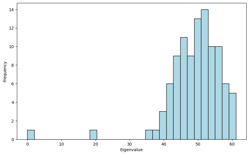
The first two eigenvalues are close to \(0\) and \(0.2 \cdot 100 = 20\) as expected. The rest of the eigenvalues are centered around \( (0.2 + 0.8) 100 /2 = 50\), but they are quite spread out, with a density resembling a half-circle. This is related to Wigner’s semicircular law which plays a key role in random matrix theory.

\(\unlhd\)

5.8.2.2. Weyl’s inequality

We prove an inequality on the sensitivity of eigenvalues which is useful in certain applications.

For a symmetric matrix \(C \in \mathbb{R}^{d \times d}\), we let \(\lambda_j(C)\), \(j=1, \ldots, d\), be the eigenvalues of \(C\) in non-increasing order with corresponding orthonormal eigenvectors \(\mathbf{v}_j\), \(j=1, \ldots, d\). The following lemma is one version of what is known as Weyl’s Inequality.

LEMMA (Weyl) Let \(A \in \mathbb{R}^{d \times d}\) and \(B \in \mathbb{R}^{d \times d}\) be symmetric matrices. Then, for all \(j=1, \ldots, d\),

\[ \max_{j \in [d]} \left|\lambda_j(B) - \lambda_j(A)\right| \leq \|B- A\|_2 \]

where \(\|C\|_2\) is the induced \(2\)-norm of \(C\). \(\flat\)

Proof idea: We use the extremal characterization of the eigenvalues together with a dimension argument.

Proof: For a symmetric matrix \(C \in \mathbb{R}^{d \times d}\), define the subspaces

\[ \mathcal{V}_k(C) = \mathrm{span}(\mathbf{v}_1, \ldots, \mathbf{v}_k) \quad\text{and}\quad \mathcal{W}_{d-k+1}(C) = \mathrm{span}(\mathbf{v}_k, \ldots, \mathbf{v}_d) \]

where \(\mathbf{v}_1,\ldots,\mathbf{v}_d\) form an orthonormal basis of eigenvectors of \(C\). Let \(H = B - A\). We prove only the upper bound. The other direction follows from interchanging the roles of \(A\) and \(B\). Because

\[ \mathrm{dim}(\mathcal{V}_j(B)) + \mathrm{dim}(\mathcal{W}_{d-j+1}(A)) = j + (d-j+1) = d+1 \]

it it can be shown (Try it!) that

\[ \mathrm{dim}\left(\mathcal{V}_j(B) \cap \mathcal{W}_{d-j+1}(A)\right) \geq d+1 - d = 1. \]

Hence the \(\mathcal{V}_j(B) \cap \mathcal{W}_{d-j+1}(A)\) is non-empty. Let \(\mathbf{v}\) be a unit vector in that intersection.

By Courant-Fischer,

\[ \lambda_j(B) \leq \langle \mathbf{v}, (A+H) \mathbf{v}\rangle = \langle \mathbf{v}, A \mathbf{v}\rangle + \langle \mathbf{v}, H \mathbf{v}\rangle \leq \lambda_j(A) + \langle \mathbf{v}, H \mathbf{v}\rangle. \]

Moreover, by Cauchy-Schwarz, since \(\|\mathbf{v}\|=1\)

\[ \langle \mathbf{v}, H \mathbf{v}\rangle \leq \|\mathbf{v}\| \|H\mathbf{v}\| \leq \|H\|_2 \]

which proves the claim. \(\square\)

5.8.2.3. Weighted case

The concepts we have introduced can also be extended to weighted graphs, that is, graphs with weights on the edges. These weights might be a measure of the strength of the connection for instance. In this section, we briefly describe this extension, which is the basis for a discrete calculus.

DEFINITION (Weighted Graph or Digraph) A weighted graph (or weighted digraph) is a triple \(G = (V, E, w)\) where \((V, E)\) is a graph (or directed graph) and \(w : E \to \mathbb{R}_+\) is a function that assigns positive real weights to the edges. For ease of notation, we write \(w_e = w_{ij} = w(i,j)\) for the weight of edge \(e = \{i,j\}\) (or \(e = (i,j)\) in the directed case). \(\natural\)

As we did for graphs, we denote the vertices \(\{1,\ldots, n\}\) and the edges \(\{e_1,\ldots, e_{m}\}\), where \(n = |V|\) and \(m =|E|\). Properties of graphs can be generalized naturally. For instance, one defines the degree of a vertex \(i\) as, in the undirected case,

\[ \delta(i) = \sum_{j:\{i,j\} \in E} w_{ij}. \]

Similarly, in the directed case, the out-degree and in-degree are

\[ \delta^+(i) = \sum_{j: (i,j) \in E} w_{ij} \qquad \text{and} \qquad \delta^+(i) = \sum_{j: (j,i) \in E} w_{ij}. \]

In the undirected case, the adjacency matrix is generalized as follows. (A similar generalization holds for the directed case.)

DEFINITION (Adjacency Matrix for Weighted Graph) Let \(G = (V, E, w)\) be a weighted graph with \(n = |V|\) vertices. The adjacency matrix \(A\) of \(G\) is the \(n\times n\) symmetric matrix defined as

\[\begin{align*} A_{ij} = \begin{cases} w_{ij} & \text{if $\{i,j\} \in E$}\\ 0 & \text{o.w.} \end{cases} \end{align*}\]

\(\natural\)

A similar generalization holds for the directed case.

DEFINITION (Adjacency Matrix for Weighted Digraph) Let \(G = (V, E, w)\) be a weighted digraph with \(n = |V|\) vertices. The adjacency matrix \(A\) of \(G\) is the \(n\times n\) matrix defined as

\[\begin{align*} A_{ij} = \begin{cases} w_{ij} & \text{if $(i,j) \in E$}\\ 0 & \text{o.w.} \end{cases} \end{align*}\]

\(\natural\)

Laplacian matrix for weighted graphs In the case of a weighted graph, the Laplacian can then be defined as follows.

DEFINITION (Laplacian for Weighted Graph) Let \(G = (V, E, w)\) be a weighted graph with \(n = |V|\) vertices and adjacency matrix \(A\). Let \(D = \mathrm{diag}(\delta(1), \ldots, \delta(n))\) be the weighted degree matrix. The Laplacian matrix associated to \(G\) is defined as \(L = D - A\). \(\natural\)

It can be shown (Try it!) that the Laplacian quadratic form satisfies in the weighted case

\[ \langle \mathbf{x}, L \mathbf{x} \rangle = \sum_{\{i,j\} \in E} w_{ij} (x_i - x_j)^2 \]

for \(\mathbf{x} = (x_1,\ldots,x_n) \in \mathbb{R}^n\).

As a positive semidefinite matrix (Exercise: Why?), the weighted Laplacian has an orthonormal basis of eigenvectors with nonnegative eigenvalues that satisfy the variational characterization we derived above. In particular, if we denote the eigenvalues \(0 = \mu_1 \leq \mu_2 \leq \cdots \leq \mu_n\), it follows from Courant-Fischer that

\[ \mu_2 = \min\left\{ \sum_{\{u, v\} \in E} w_{uv} (x_u - x_v)^2 \,:\, \mathbf{x} = (x_1, \ldots, x_n) \in \mathbb{R}^n, \sum_{u=1}^n x_u = 0, \sum_{u = 1}^n x_u^2 = 1 \right\}. \]

If we generalize the cut ratio as

\[ \phi(S) = \frac{\sum_{i \in S, j \in S^c} w_{ij}}{\min\{|S|, |S^c|\}} \]

for \(\emptyset \neq S \subset V\) and let

\[ \phi_G = \min\left\{ \phi(S)\,:\, \emptyset \neq S \subset V \right\} \]

it can be shown (Try it!) that

\[ \mu_2 \leq 2 \phi_G \]

as in the unweighted case.

Normalized Laplacian Other variants of the Laplacian matrix have also been studied. We introduced the normalized Laplacian next. Recall that in the weighted case, the degree is defined as \(\delta(i) = \sum_{j:\{i,j\} \in E} w_{i,j}\).

DEFINITION (Normalized Laplacian) The normalized Laplacian of \(G = (V,E,w)\) with adjacency matrix \(A\) and degree matrix \(D\) is defined as

\[ \mathcal{L} = I - D^{-1/2} A D^{-1/2}. \]

\(\natural\)

Using our previous observations about multiplication by diagonal matrices, the entries of \(\mathcal{L}\) are

\[ (\mathcal{L})_{i,j} = (I - (D^{-1/2} A D^{-1/2})_{i,j} = 1 - \frac{a_{i,j}}{\sqrt{\delta(i) \delta(j)}}. \]

We also note the following relation to the Laplacian matrix:

\[ \mathcal{L} = D^{-1/2} L D^{-1/2}. \]

We check that the normalized Laplacian is symmetric:

\[\begin{align*} \mathcal{L}^T &= I^T - (D^{-1/2} A D^{-1/2})^T\\ &= I - (D^{-1/2})^T A^T (D^{-1/2})^T\\ &= I - D^{-1/2} A D^{-1/2}\\ &= \mathcal{L}. \end{align*}\]

It is also positive semidefinite. Indeed,

\[ \mathbf{x}^T \mathcal{L} \mathbf{x} = \mathbf{x}^T D^{-1/2} L D^{-1/2} \mathbf{x} = (D^{-1/2} \mathbf{x})^T L (D^{-1/2} \mathbf{x}) \geq 0, \]

by the properties of the Laplacian matrix.

Hence by the Spectral Theorem, we can write

\[ \mathcal{L} = \sum_{i=1}^n \eta_i \mathbf{z}_i \mathbf{z}_i^T, \]

where the \(\mathbf{z}_i\)s are orthonormal eigenvectors of \(\mathcal{L}\) and the eigenvalues satisfy \(0 \leq \eta_1 \leq \eta_2 \leq \cdots \leq \eta_n\).

One more observation: because the constant vector is eigenvector of \(L\) with eigenvalue \(0\), we get that \(D^{1/2} \mathbf{1}\) is an eigenvector of \(\mathcal{L}\) with eigenvalue \(0\). So \(\eta_1 = 0\) and we set

\[ (\mathbf{z}_1)_i = \left(\frac{D^{1/2} \mathbf{1}}{\|D^{1/2} \mathbf{1}\|_2}\right)_i = \sqrt{\frac{\delta(i)}{\sum_{i\in V} \delta(i)}}, \quad \forall i \in [n], \]

which makes \(\mathbf{z}_1\) into a unit norm vector.

The relationship to the Laplacian matrix immediately implies (prove it!) that

\[ \mathbf{x}^T \mathcal{L} \mathbf{x} = \sum_{\{i,j\} \in E} w_{ij} \left(\frac{x_i}{\sqrt{\delta(i)}} - \frac{x_j}{\sqrt{\delta(j)}}\right)^2, \]

for \(\mathbf{x} = (x_1,\ldots,x_n)^T \in \mathbb{R}^n\).

Through the change of variables

\[ y_i = \frac{x_i}{\sqrt{\delta(i)}}, \]

Courant-Fischer gives this time (Why?)

\[ \eta_2 = \min\left\{ \sum_{\{u, v\} \in E} w_{uv} (y_u - y_v)^2 \,:\, \mathbf{y} = (y_1, \ldots, y_n)^T \in \mathbb{R}^n, \sum_{u=1}^n \delta(u) y_u = 0, \sum_{u = 1}^n \delta(u) y_u^2 = 1 \right\}. \]

For a subset of vertices \(S \subseteq V\), let

\[ |S|_w = \sum_{i \in S} \delta(i), \]

which we refer to as the volume of \(S\). It is measure of the size of \(S\) weighted by the degrees.

If we consider the normalized cut ratio, or bottleneck ratio,

\[ \phi^N(S) = \frac{\sum_{i \in S, j \in S^c} w_{ij}}{\min\{|S|_w, |S^c|_w\}} \]

for \(\emptyset \neq S \subset V\) and let

\[ \phi^N_G = \min\left\{ \phi^N(S)\,:\, \emptyset \neq S \subset V \right\} \]

it can be shown (Try it!) that

\[ \eta_2 \leq 2 \phi^N_G. \]

The normalized cut ratio is similar to the cut ratio, except that the notion of balance of the cut is measured in terms of volume. Note that this concept is also useful in the unweighted case.

We will an application of the normalized Laplacian later in this chapter.

5.8.2.4. Image segmentation

We give a different, more involved application of the ideas developed in this topic to image segmentation. Let us quote Wikipedia:

In computer vision, image segmentation is the process of partitioning a digital image into multiple segments (sets of pixels, also known as image objects). The goal of segmentation is to simplify and/or change the representation of an image into something that is more meaningful and easier to analyze. Image segmentation is typically used to locate objects and boundaries (lines, curves, etc.) in images. More precisely, image segmentation is the process of assigning a label to every pixel in an image such that pixels with the same label share certain characteristics.

Throughout, we will use the scikit-image library for processing images.

from skimage import io, segmentation, color
from skimage import graph
from sklearn.cluster import KMeans

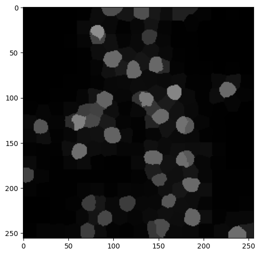
As an example, here is a picture of cell nuclei taken through optical microscopy as part of some medical experiment. It is taken from here. Here we used the function skimage.io.imread to load an image from file.

img = io.imread('cell-nuclei.png')
fig, ax = plt.subplots(figsize=(6, 6))
ax.imshow(img)
plt.show()

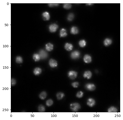
Suppose that, as part of this experiment, we have a large number of such images and need to keep track of the cell nuclei in some way (maybe count how many there are, or track them from frame to frame). A natural pre-processing step is to identify the cell nuclei in the image. We use image segmentation for this purpose.

We will come back to the example below. Let us start with some further examples.

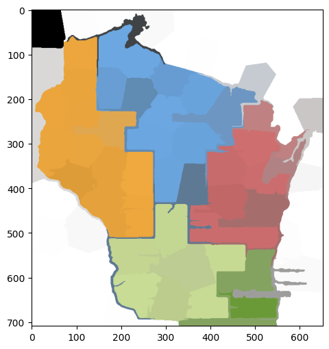
We will first work with the following map of Wisconsin regions.

img = io.imread('wisconsin-regions.png')
fig, ax = plt.subplots(figsize=(6, 6))
ax.imshow(img)
plt.show()

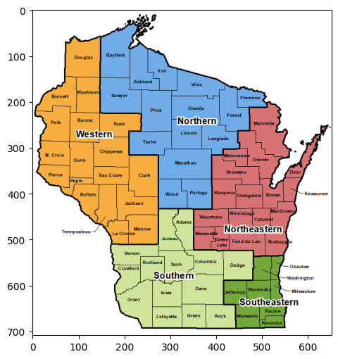
A color image such as this one is encoded as a \(3\)-dimensional array (or tensor), meaning that it is an array with \(3\) indices (unlike matrices which have only two indices).

img.shape

(709, 652, 3)

The first two indices capture the position of a pixel. The third index capture the RGB color model. Put differently, each pixel in the image has three numbers (between 0 and 255) attached to it that encodes its color.

For instance, at position \((300,400)\) the RGB color is:

img[300,400,:]

array([111, 172, 232], dtype=uint8)

plt.imshow(np.reshape(img[300,400,:],(1,1,3)))
plt.show()

To perform image segmentation using the spectral graph theory we have developed, we transform our image into a graph.

The first step is to coarsen the image by creating super-pixels, or regions of pixels that are close and have similar color. For this purpose, we will use skimage.segmentation.slic, which in essence uses \(k\)-means clustering on the color space to identify blobs of pixels that are in close proximity and have similar colors. It takes as imput a number of super-pixels desired (n_segments), a compactness parameter (compactness) and a smoothing parameter (sigma). The output is a label assignment for each pixel in the form of a \(2\)-dimensional array.

On the choice of the parameter compactness via scikit-image:

Balances color proximity and space proximity. Higher values give more weight to space proximity, making superpixel shapes more square/cubic. This parameter depends strongly on image contrast and on the shapes of objects in the image. We recommend exploring possible values on a log scale, e.g., 0.01, 0.1, 1, 10, 100, before refining around a chosen value.

The parameter sigma controls the level of blurring applied to the image as a pre-processing step. In practice, experimentation is required to choose good parameters.

labels1 = segmentation.slic(img, 
                            compactness=25, 
                            n_segments=100, 
                            sigma=2., 
                            start_label=0)
print(labels1)

[[ 0  0  0 ...  8  8  8]
 [ 0  0  0 ...  8  8  8]
 [ 0  0  0 ...  8  8  8]
 ...
 [77 77 77 ... 79 79 79]
 [77 77 77 ... 79 79 79]
 [77 77 77 ... 79 79 79]]

A neat way to vizualize the super-pixels is to use the function skimage.color.label2rgb which takes as input an image and an array of labels. In the mode kind='avg', it outputs a new image where the color of each pixel is replaced with the average color of its label (that is, the average of the RGB color over all pixels with the same label). As they say, an image is worth a thousand words - let’s just see what it does.

out1 = color.label2rgb(labels1, img/255, kind='avg', bg_label=0)
out1.shape

(709, 652, 3)

fig, ax = plt.subplots(figsize=(6, 6))
ax.imshow(out1)
plt.show()

Recall that our goal is to turn our original image into a graph. After the first step of creating super-pixels, the second step is to form a graph whose nodes are the super-pixels. Edges are added between adjacent super-pixels and a weight is given to each edge which reflects the difference in mean color between the two.

We use skimage.graph.rag_mean_color. In mode similarity, it uses the following weight formula (quoting the documentation):

The weight between two adjacent regions is exp(-d^2/sigma) where d=|c1-c2|, where c1 and c2 are the mean colors of the two regions. It represents how similar two regions are.

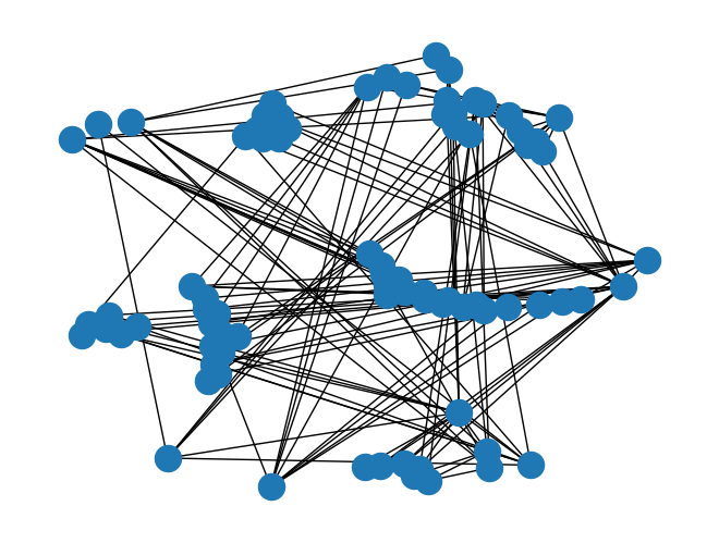
The output, which is known as a region adjacency graph (RAG), is a NetworkX graph and can be manipulated using that package.

g = graph.rag_mean_color(img, labels1, mode='similarity')
nx.draw(g, pos=nx.spring_layout(g))

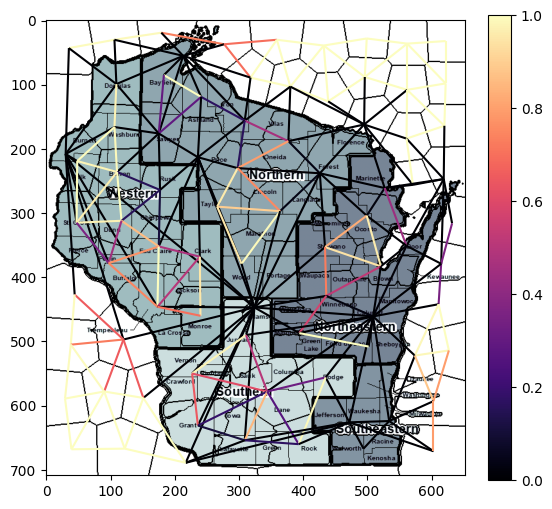
scikit-image also provides a more effective way of vizualizing a RAG, using the function skimage.future.graph.show_rag. Here the graph is super-imposed on the image and the edge weights are depicted by their color.

fig, ax = plt.subplots(nrows=1, figsize=(6, 8))
lc = graph.show_rag(labels1, g, img, ax=ax)
fig.colorbar(lc, fraction=0.05, ax=ax)
plt.show()

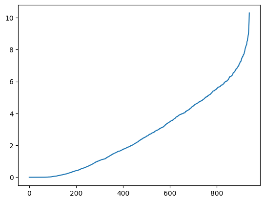
We can apply the spectral clustering techniques we have developed in this chapter. Next we compute a spectral decomposition of the weighted Laplacian and plot the eigenvalues.

L = nx.laplacian_matrix(g).toarray()
print(L)

[[ 9.93627574e-01 -9.93627545e-01  0.00000000e+00 ...  0.00000000e+00
   0.00000000e+00  0.00000000e+00]
 [-9.93627545e-01  1.98331432e+00 -9.89686777e-01 ...  0.00000000e+00
   0.00000000e+00  0.00000000e+00]
 [ 0.00000000e+00 -9.89686777e-01  1.72084919e+00 ...  0.00000000e+00
   0.00000000e+00  0.00000000e+00]
 ...
 [ 0.00000000e+00  0.00000000e+00  0.00000000e+00 ...  4.03242708e-05
   0.00000000e+00  0.00000000e+00]
 [ 0.00000000e+00  0.00000000e+00  0.00000000e+00 ...  0.00000000e+00
   7.93893423e-01  0.00000000e+00]
 [ 0.00000000e+00  0.00000000e+00  0.00000000e+00 ...  0.00000000e+00
   0.00000000e+00  1.99992197e+00]]

w, v = LA.eigh(L)
plt.plot(np.sort(w))
plt.show()

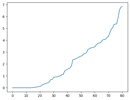
From the theory, this suggests that there are roughly 15 components in this graph. We project to \(15\) dimensions and apply \(k\)-means clustering to find segments. Rather than using our own implementation, we use sklearn.cluster.KMeans from the scikit-learn library. That implementation uses the \(k\)-means\(++\) initialization, which is particularly effective in practice. A label assignment for each node can be accessed using labels_.

ndims = 15 # number of dimensions to project to
nsegs = 10 # number of segments

top = np.argsort(w)[1:ndims]
topvecs = v[:,top]
topvals = w[top]

kmeans = KMeans(n_clusters=nsegs, random_state=12345).fit(topvecs)
assign_seg = kmeans.labels_
print(assign_seg)

[1 1 1 1 1 1 1 1 1 2 9 1 1 2 1 1 1 9 8 1 9 6 9 2 1 9 1 9 2 9 9 2 2 4 1 2 9
 9 2 4 3 2 4 4 2 2 9 2 4 3 1 5 2 4 3 4 2 0 5 4 5 3 3 4 0 0 0 5 5 1 5 1 3 0
 0 0 5 5 7 3 5]

To vizualize the segmentation, we assign to each segment (i.e., collection of super-pixels) a random color. This can be done using skimage.color.label2rgb again, this time in mode kind='overlay'. First, we assign to each pixel from the original image its label under this clustering. Recall that labels1 assigns to each pixel its super-pixel (represented by a node of the RAG), so that applying assign_seg element-wise to labels1 results is assigning a cluster to each pixel. In code:

labels2 = assign_seg[labels1]
print(labels2)

[[1 1 1 ... 1 1 1]
 [1 1 1 ... 1 1 1]
 [1 1 1 ... 1 1 1]
 ...
 [5 5 5 ... 3 3 3]
 [5 5 5 ... 3 3 3]
 [5 5 5 ... 3 3 3]]

out2 = color.label2rgb(labels2, kind='overlay', bg_label=0)
out2.shape

(709, 652, 3)

fig, ax = plt.subplots(nrows=2, sharex=True, sharey=True, figsize=(16, 8))
ax[0].imshow(img)
ax[1].imshow(out2)
plt.show()

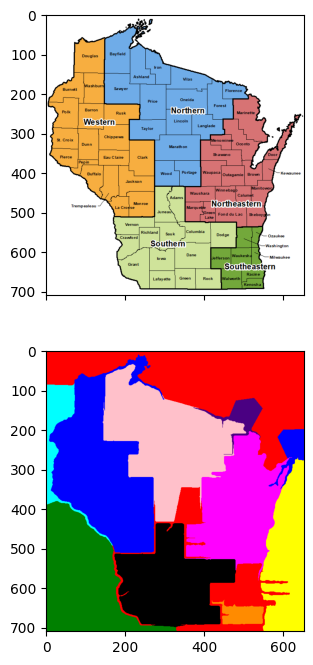
As you can see, the result is reasonable but far from perfect.

For ease of use, we encapsulate the main steps above in sub-routines.

def imgseg_rag(img, compactness=30, n_spixels=400, sigma=0., figsize=(10,10)):
    labels1 = segmentation.slic(img, 
                                compactness=compactness, 
                                n_segments=n_spixels, 
                                sigma=sigma, 
                                start_label=0)
    out1 = color.label2rgb(labels1, img/255, kind='avg', bg_label=0)
    g = graph.rag_mean_color(img, labels1, mode='similarity')
    fig, ax = plt.subplots(figsize=figsize)
    ax.imshow(out1)
    plt.show()
    return labels1, g

def imgseg_eig(g):
    L = nx.laplacian_matrix(g).toarray()
    w, v = LA.eigh(L)
    plt.plot(np.sort(w))
    plt.show()
    return w,v

def imgseg_labels(w, v, n_dims=10, n_segments=5, random_state=0):
    top = np.argsort(w)[1:n_dims]
    topvecs = v[:,top]
    topvals = w[top]
    kmeans = KMeans(n_clusters=n_segments, 
                    random_state=random_state).fit(topvecs)
    assign_seg = kmeans.labels_
    labels2 = assign_seg[labels1]
    return labels2

def imgseg_viz(img, labels2, figsize=(20,10)):
    out2 = color.label2rgb(labels2, kind='overlay', bg_label=0)
    fig, ax = plt.subplots(nrows=2, sharex=True, sharey=True, figsize=figsize)
    ax[0].imshow(img)
    ax[1].imshow(out2)
    plt.show()

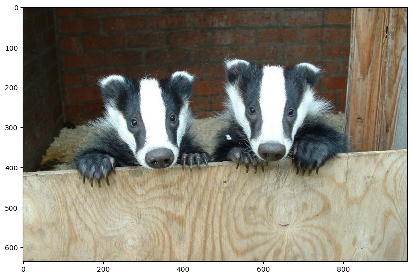
Let’s try a more complicated image. This one is taken from here.

img = io.imread('two-badgers.jpg')
fig, ax = plt.subplots(figsize=(10, 10))
ax.imshow(img)
plt.show()

Recall that the choice of parameters requires significant fidgeting.

labels1, g = imgseg_rag(img, 
                        compactness=30, 
                        n_spixels=1000, 
                        sigma=0., 
                        figsize=(10,10))

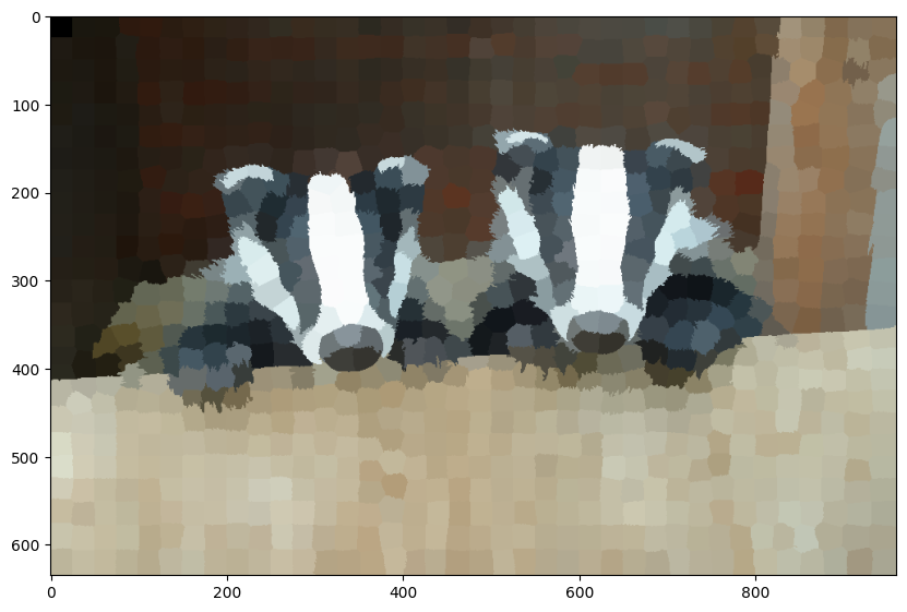
w, v = imgseg_eig(g)

labels2 = imgseg_labels(w, v, n_dims=60, n_segments=50, random_state=535)
imgseg_viz(img,labels2,figsize=(20,10))

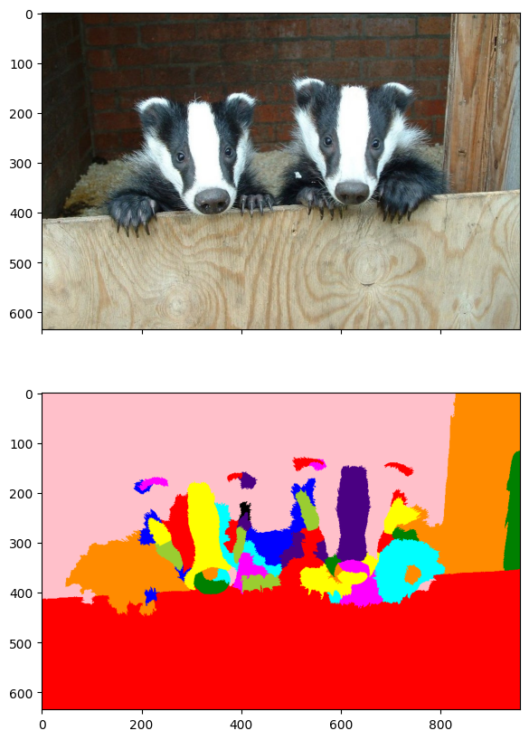
Again, the results are far from perfect - but not unreasonable.

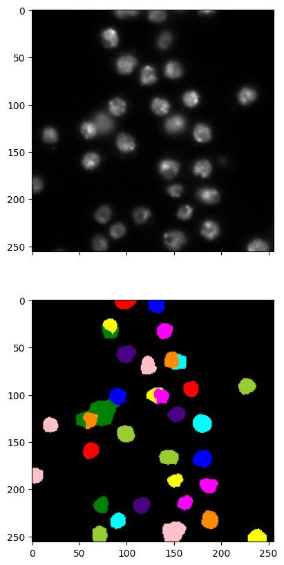
Finally, we return to our medical example. We first reload the image and find super-pixels.

img = io.imread('cell-nuclei.png')
labels1, g = imgseg_rag(img,compactness=40,n_spixels=300,sigma=0.1,figsize=(6,6))

We then form the weighted Laplacian and plot its eigenvalues. This time, about \(40\) dimensions seem appropriate.

w, v = imgseg_eig(g)

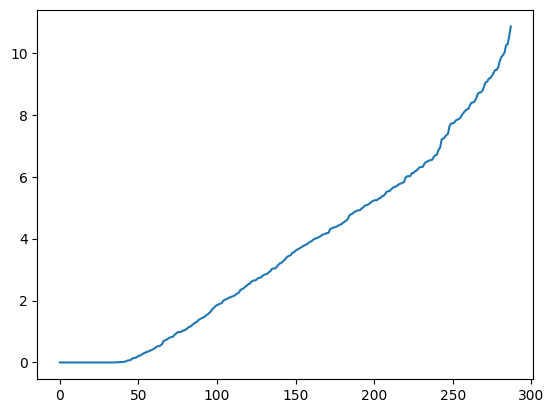
labels2 = imgseg_labels(w, v, n_dims=40, n_segments=30, random_state=535)
imgseg_viz(img,labels2,figsize=(20,10))

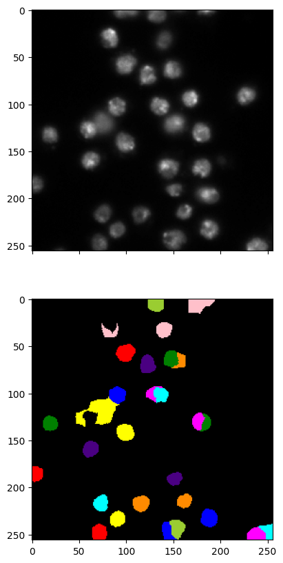
This method is quite finicky. The choice of parameters affects the results significantly. You should see for yourself.

We mention that scikit-image has an implementation of a closely related method, Normalized Cut, skimage.graph.cut_normalized. Rather than performing \(k\)-means after projection, it recursively performs \(2\)-way cuts on the RAG and resulting subgraphs.

We try it next. The results are similar as you can see.

labels2 = graph.cut_normalized(labels1, g)
imgseg_viz(img,labels2,figsize=(20,10))

There are many other image segmentation methods. See for example here.