\(\newcommand{\bmu}{\boldsymbol{\mu}}\) \(\newcommand{\bSigma}{\boldsymbol{\Sigma}}\) \(\newcommand{\bfbeta}{\boldsymbol{\beta}}\) \(\newcommand{\bflambda}{\boldsymbol{\lambda}}\) \(\newcommand{\bgamma}{\boldsymbol{\gamma}}\) \(\newcommand{\bsigma}{{\boldsymbol{\sigma}}}\) \(\newcommand{\bpi}{\boldsymbol{\pi}}\) \(\newcommand{\btheta}{{\boldsymbol{\theta}}}\) \(\newcommand{\bphi}{\boldsymbol{\phi}}\) \(\newcommand{\balpha}{\boldsymbol{\alpha}}\) \(\newcommand{\blambda}{\boldsymbol{\lambda}}\) \(\renewcommand{\P}{\mathbb{P}}\) \(\newcommand{\E}{\mathbb{E}}\) \(\newcommand{\indep}{\perp\!\!\!\perp} \newcommand{\bx}{\mathbf{x}}\) \(\newcommand{\bp}{\mathbf{p}}\) \(\renewcommand{\bx}{\mathbf{x}}\) \(\newcommand{\bX}{\mathbf{X}}\) \(\newcommand{\by}{\mathbf{y}}\) \(\newcommand{\bY}{\mathbf{Y}}\) \(\newcommand{\bz}{\mathbf{z}}\) \(\newcommand{\bZ}{\mathbf{Z}}\) \(\newcommand{\bw}{\mathbf{w}}\) \(\newcommand{\bW}{\mathbf{W}}\) \(\newcommand{\bv}{\mathbf{v}}\) \(\newcommand{\bV}{\mathbf{V}}\) \(\newcommand{\bfg}{\mathbf{g}}\) \(\newcommand{\bfh}{\mathbf{h}}\) \(\newcommand{\horz}{\rule[.5ex]{2.5ex}{0.5pt}}\) \(\renewcommand{\S}{\mathcal{S}}\) \(\newcommand{\X}{\mathcal{X}}\) \(\newcommand{\var}{\mathrm{Var}}\) \(\newcommand{\pa}{\mathrm{pa}}\) \(\newcommand{\Z}{\mathcal{Z}}\) \(\newcommand{\bh}{\mathbf{h}}\) \(\newcommand{\bb}{\mathbf{b}}\) \(\newcommand{\bc}{\mathbf{c}}\) \(\newcommand{\cE}{\mathcal{E}}\) \(\newcommand{\cP}{\mathcal{P}}\) \(\newcommand{\bbeta}{\boldsymbol{\beta}}\) \(\newcommand{\bLambda}{\boldsymbol{\Lambda}}\) \(\newcommand{\cov}{\mathrm{Cov}}\) \(\newcommand{\bfk}{\mathbf{k}}\) \(\newcommand{\idx}[1]{}\) \(\newcommand{\xdi}{}\)
5.4. Spectral properties of the Laplacian matrix#
In this section, we look at the spectral properties of the Laplacian of a graph.
5.4.1. Eigenvalues of the Laplacian matrix: first observations#
Let \(G = (V, E)\) be a graph with \(n = |V|\) vertices. Two observations:
1- Since the Laplacian matrix \(L\) of \(G\) is symmetric, by the Spectral Theorem, it has a spectral decomposition
where the \(\mathbf{y}_i\)’s form an orthonormal basis of \(\mathbb{R}^n\).
2- Further, because \(L\) is positive semidefinite, the eigenvalues are nonnegative. By convention, we assume
Note that this is the opposite order to we used in the previous section.
Another observation:
LEMMA Let \(G = (V, E)\) be a graph with \(n = |V|\) vertices and Laplacian matrix \(L\). The constant unit vector
is an eigenvector of \(L\) with eigenvalue \(0\). \(\flat\)
Proof: Let \(B\) be an oriented incidence matrix of \(G\) recall that \(L = B B^T\). By construction \(B^T \mathbf{y}_1 = \mathbf{0}\) since each column of \(B\) has exactly one \(1\) and one \(-1\). So \(L \mathbf{y}_1 = B B^T \mathbf{y}_1 = \mathbf{0}\) as claimed. \(\square\)
In general, the constant vector may not be the only eigenvector with eigenvalue one.
NUMERICAL CORNER: One use of the spectral decomposition of the Laplacian matrix is in graph drawing\(\idx{graph drawing}\xdi\). We illustrate this next. Given a graph \(G = (V, E)\), it is not clear a priori how to draw it in the plane since the only information available are adjacencies of vertices. One approach is just to position the vertices at random. The function networkx.draw or networkx.draw_networkx can take as input different graph layout functions that return an \(x\) and \(y\)-coordinate for each vertex.
We will test this on a grid graph. We use networkx.grid_2d_graph to construct such a graph.
G = nx.grid_2d_graph(4,7)
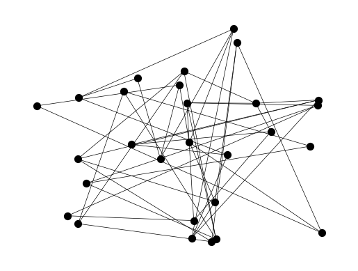
One layout approach is to choose random locations for the nodes. Specifically, for every node, a position is generated by choosing each coordinate uniformly at random on the interval \([0,1]\).
nx.draw_networkx(G, pos=nx.random_layout(G, seed=535), with_labels=False,
                 node_size=50, node_color='black', width=0.5)
plt.axis('off')
plt.show()

Clearly, this is hard to read.
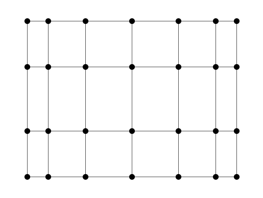
Another approach is to map the vertices to two eigenvectors, similarly to what we did for dimensionality reduction. The eigenvector associated to \(\mu_1\) is constant and therefore not useful for drawing. We try the next two. We use the Laplacian matrix. This is done using networkx.spectral_layout.
nx.draw_networkx(G, pos=nx.spectral_layout(G), with_labels=False,
                 node_size=50, node_color='black', width=0.5)
plt.axis('off')
plt.show()

Interestingly, the outcome is provides a much more natural drawing of the graph, revealing its underlying structure as a grid. We will come back later to try to explain this, after we have developed further understanding of the spectral properties of the Laplacian matrix.
\(\unlhd\)
5.4.2. Laplacian matrix and connectivity#
As we indicated before, the Laplacian matrix contains information about the connectedness of \(G\). We elaborate on a first concrete connection here. But first we will need a useful form of the Laplaican quadratic form \(\mathbf{x}^T L \mathbf{x}\) which enters in the variational charaterization of the eigenvalues.
LEMMA (Laplacian Quadratic Form) \(\idx{Laplacian quadratic form lemma}\xdi\) Let \(G = (V, E)\) be a graph with \(n = |V|\) vertices and Laplacian matrix \(L\). We have the following formula for the Laplacian quadratic form
for any \(\mathbf{x} = (x_1, \ldots, x_n) \in \mathbb{R}^n\). \(\flat\)
Here is an intuitive way of interpreting this lemma. If one thinks of \(\mathbf{x} = (x_1, \ldots, x_n) \in \mathbb{R}^n\) as a real-valued function over the vertices (i.e., it associates a real value \(x_i\) to vertex \(i\) for each \(i\)), then the Laplacian quadratic form measures how “smooth” the function is over the graph in the following sense. A small value of \(\mathbf{x}^T L \mathbf{x}\) indicates that adjacent vertices tend to get assigned close values.
Proof: Let \(B\) be an oriented incidence matrix of \(G\). We have that \(L = B B^T\). Thus, for any \(\mathbf{x}\), we have \((B^T \mathbf{x})_k = x_v - x_u\) if the edge \(e_k = \{u, v\}\) is oriented as \((u,v)\) under \(B\). That implies
Since the latter is always nonnegative, it also implies that \(L\) is positive semidefinite. \(\square\)
We are now ready to derive connectivity consequences. Recall that, for any graph \(G\), the Laplacian eigenvalue \(\mu_1 = 0\).
LEMMA (Laplacian and Connectivity) \(\idx{Laplacian and connectivity lemma}\xdi\) If \(G\) is connected, then the Laplacian eigenvalue \(\mu_2 > 0\). \(\flat\)
Proof: Let \(G = (V, E)\) with \(n = |V|\) and let \(L = \sum_{i=1}^n \mu_i \mathbf{y}_i \mathbf{y}_i^T\) be a spectral decomposition of its Laplacian \(L\) with \(0 = \mu_1 \leq \cdots \leq \mu_n\). Suppose by way of contradiction that \(\mu_2 = 0\). Any eigenvector \(\mathbf{y} = (y_{1}, \ldots, y_{n})\) with \(0\) eigenvalue satisfies \(L \mathbf{y} = \mathbf{0}\) by definition. By the Laplacian Quadratic Form Lemma then
1- In order for this to hold, it must be that any two adjacent vertices \(i\) and \(j\) have \(y_{i} = y_{j}\). That is, \(\{i,j\} \in E\) implies \(y_i = y_j\).
2- Furthermore, because \(G\) is connected, between any two of its vertices \(u\) and \(v\) - adjacent or not - there is a path \(u = w_0 \sim \cdots \sim w_k = v\) along which the \(y_{w}\)’s must be the same. Thus \(\mathbf{y}\) is a constant vector.
But that is a contradiction since the eigenvectors \(\mathbf{y}_1, \ldots, \mathbf{y}_n\) are in fact linearly independent, so that \(\mathbf{y}_1\) and \(\mathbf{y}_2\) cannot both be a constant vector. \(\square\)
The quantity \(\mu_2\) is sometimes referred to as the algebraic connectivity\(\idx{algebraic connectivity}\xdi\) of the graph. The corresponding eigenvector, \(\mathbf{y}_2\), is known as the Fiedler vector\(\idx{Fiedler vector}\xdi\).
We state the following (more general) converse result without proof.
LEMMA If \(\mu_{k+1}\) is the smallest nonzero Laplacian eigenvalue of \(G\), then \(G\) has \(k\) connected components. \(\flat\)
We will be interested in more quantitative results of this type. Before proceeding, we start with a simple observation. By our proof of the Spectral Theorem, the largest eigenvalue \(\mu_n\) of the Laplacian matrix \(L\) is the solution to the optimization problem
Such extremal characterization is useful in order to bound the eigenvalue \(\mu_n\), since any choice of \(\mathbf{x}\) with \(\|\mathbf{x}\| =1\) gives a lower bound through the quantity \(\langle \mathbf{x}, L \mathbf{x}\rangle\). That perspective will be key to our application to graph partitioning.
For now, we give a simple consequence.
LEMMA (Laplacian and Maximum Degree) \(\idx{Laplacian and maximum degree lemma}\xdi\) Let \(G = (V, E)\) be a graph with maximum degree \(\bar{\delta}\). Let \(\mu_n\) be the largest eigenvalue of its Laplacian matrix \(L\). Then
\(\flat\)
Proof idea: As explained before the statement of the lemma, for the lower bound it suffices to find a good test unit vector \(\mathbf{x}\) to plug into \(\langle \mathbf{x}, L \mathbf{x}\rangle\). A clever choice does the trick.
Proof: We start with the lower bound. Let \(u \in V\) be a vertex with degree \(\bar{\delta}\). Let \(\mathbf{z}\) be the vector with entries
and let \(\mathbf{x}\) be the unit vector \(\mathbf{z}/\|\mathbf{z}\|\). By definition of the degree of \(u\), \(\|\mathbf{z}\|^2 = \bar{\delta}^2 + \bar{\delta}(-1)^2 = \bar{\delta}(\bar{\delta}+1)\). Using the Laplacian Quadratic Form Lemma,
where we restricted the sum to those edges incident with \(u\) and used the fact that all terms in the sum are nonnegative. Finally
so that
as claimed.
We proceed with the lower bound. For any unit vector \(\mathbf{x}\),
By the Cauchy-Schwarz inequality, this is
\(\square\)
NUMERICAL CORNER: We construct a graph with two connected components and check the results above. We work directly with the adjacency matrix.
A = np.array([[0, 1, 1, 0, 0],
              [1, 0, 1, 0, 0],
              [1, 1, 0, 0, 0],
              [0, 0, 0, 0, 1],
              [0, 0, 0, 1, 0]])
print(A)
[[0 1 1 0 0]
 [1 0 1 0 0]
 [1 1 0 0 0]
 [0 0 0 0 1]
 [0 0 0 1 0]]
Note the block structure.
The degrees can be obtained by summing the rows of the adjacency matrix.
degrees = A.sum(axis=1)
print(degrees)
[2 2 2 1 1]
D = np.diag(degrees)
print(D)
[[2 0 0 0 0]
 [0 2 0 0 0]
 [0 0 2 0 0]
 [0 0 0 1 0]
 [0 0 0 0 1]]
L = D - A
print(L)
[[ 2 -1 -1  0  0]
 [-1  2 -1  0  0]
 [-1 -1  2  0  0]
 [ 0  0  0  1 -1]
 [ 0  0  0 -1  1]]
print(LA.eigvals(L))
[ 3.00000000e+00 -3.77809194e-16  3.00000000e+00  2.00000000e+00
  0.00000000e+00]
Observe that (up to numerical error) there are two \(0\) eigenvalues and that the largest eigenvalue is greater or equal than the maximum degree plus one.
To compute the Laplacian matrix, one can also use the function networkx.laplacian_matrix. For example, the Laplacian of the Petersen graph is the following:
G = nx.petersen_graph()
L = nx.laplacian_matrix(G).toarray()
print(L)
[[ 3 -1  0  0 -1 -1  0  0  0  0]
 [-1  3 -1  0  0  0 -1  0  0  0]
 [ 0 -1  3 -1  0  0  0 -1  0  0]
 [ 0  0 -1  3 -1  0  0  0 -1  0]
 [-1  0  0 -1  3  0  0  0  0 -1]
 [-1  0  0  0  0  3  0 -1 -1  0]
 [ 0 -1  0  0  0  0  3  0 -1 -1]
 [ 0  0 -1  0  0 -1  0  3  0 -1]
 [ 0  0  0 -1  0 -1 -1  0  3  0]
 [ 0  0  0  0 -1  0 -1 -1  0  3]]
print(LA.eigvals(L))
[ 5.00000000e+00  2.00000000e+00 -2.80861083e-17  5.00000000e+00
  5.00000000e+00  2.00000000e+00  2.00000000e+00  5.00000000e+00
  2.00000000e+00  2.00000000e+00]
\(\unlhd\)
5.4.3. Variational characterization of second Laplacian eigenvalue#
The definition \(A \mathbf{x} = \lambda \mathbf{x}\) is perhaps not the best way to understand why the eigenvectors of the Laplacian matrix are useful. Instead the following application of the Courant-Fischer theorem\(\idx{Courant-Fischer Theorem}\xdi\) provides much insight, as we will see in the rest of this chapter.
THEOREM (Variational Characterization of \(\mu_2\)) \(\idx{variational characterization of the algebraic connectivity}\xdi\) Let \(G = (V, E)\) be a graph with \(n = |V|\) vertices. Assume the Laplacian \(L\) of \(G\) has spectral decomposition \(L = \sum_{i=1}^n \mu_i \mathbf{y}_i \mathbf{y}_i^T\) with \(0 = \mu_1 \leq \mu_2 \leq \cdots \leq \mu_n\) and \(\mathbf{y}_1 = \frac{1}{\sqrt{n}}(1,\ldots,1)\). Then
Taking \(\mathbf{x} = \mathbf{y}_2\) achieves this minimum. \(\sharp\)
Proof: By the Courant-Fischer Theorem,
where \(\mathcal{V}_{n-1} = \mathrm{span}(\mathbf{y}_2, \ldots, \mathbf{y}_n) = \mathrm{span}(\mathbf{y}_1)^\perp\). Observe that, because we reverse the order of the eigenvalues compared to the convention used in the Courant-Fischer theorem, we must adapt the definition of \(\mathcal{V}_{n-1}\) slightly. Moreover we know that \(\mathcal{R}_L(\mathbf{y}_2) = \mu_2\). We make a simple transformation of the problem.
We claim that
Indeed, if \(\mathbf{u} \in \mathrm{span}(\mathbf{y}_1)^\perp\) has unit norm, i.e., \(\|\mathbf{u}\| = 1\), then
In other words, we shown that
To prove the other direction, for any \(\mathbf{u} \neq \mathbf{0}\), we can normalize it by defining \(\mathbf{x} = \mathbf{u}/\|\mathbf{u}\|\) and we note that
Moreover \(\langle \mathbf{u}, \mathbf{y}_1\rangle = 0\) if only if \(\langle \mathbf{x}, \mathbf{y}_1\rangle = 0\). That establishes \((*)\), since any objective value achieved in the original formulation can be achieved in the new one.
Using that \(\mathbf{y}_1 = \frac{1}{\sqrt{n}}(1,\ldots,1)\), the condition \(\langle \mathbf{x}, \mathbf{y}_1 \rangle = 0\), i.e., \(\sum_{i=1}^n (x_i/\sqrt{n}) = 0\), is equivalent to \(\sum_{i=1}^n x_i = 0\). Similary, the condition \(\|\mathbf{x}\|=1\) is equivalent, after squaring each side, to \(\sum_{j=1}^n x_j^2 = 1\).
Finally, the claim follows from the Laplacian Quadratic Form Lemma. \(\square\)
One application of this extremal characterization is the graph drawing heuristic we described previously. Consider the entries of the second Laplacian eigenvector \(\mathbf{y}_2\). Its entries are centered around \(0\) by the condition \(\langle \mathbf{y}_1, \mathbf{y}_2\rangle = 0\). Because it minimizes the following quantity over all centered unit vectors,
the eigenvector \(\mathbf{y}_2\) tends to assign similar coordinates to adjacent vertices. A similar reasoning applies to the third Laplacian eigenvector, which in addition is orthogonal to the second one. So coordinates based on the second and third Laplacian eigenvectors should be expected to position adjacent vertices close-by and hence minimizing the need for long-range edges in the visualization. In particular, it reveals some of the underlying Euclidean geometry of the graph, as the next example shows.
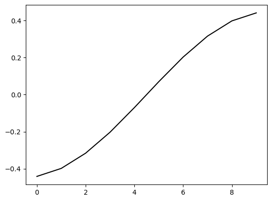
NUMERICAL CORNER: This is perhaps easiest to see on a path graph. Recall that NetworkX numbers vertices \(0,\ldots,n-1\).
G = nx.path_graph(10)
We plot the second Laplacian eigenvector (i.e., the eigenvector of the Laplacian matrix corresponding to the second smallest eigenvalue). We use numpy.argsort to find the index of the second smallest eigenvalue. Because indices start at 0, we want entry 1 of the output.
L = nx.laplacian_matrix(G).toarray()
w, v = LA.eigh(L)
y2 = v[:,np.argsort(w)[1]]

plt.plot(y2, c='k')
plt.show()

\(\unlhd\)
EXAMPLE: (Two-Component Graph) Let \(G=(V,E)\) be a graph with two connected components \(\emptyset \neq V_1, V_2 \subseteq V\). By the properties of connected components, we have \(V_1 \cap V_2 = \emptyset\) and \(V_1 \cup V_2 = V\). Assume the Laplacian \(L\) of \(G\) has spectral decomposition \(L = \sum_{i=1}^n \mu_i \mathbf{y}_i \mathbf{y}_i^T\) with \(0 = \mu_1 \leq \mu_2 \leq \cdots \leq \mu_n\) and \(\mathbf{y}_1 = \frac{1}{\sqrt{n}}(1,\ldots,1)\). We claimed earlier that for such a graph \(\mu_2 = 0\). We prove this here using the Variational Characterization of \(\mu_2\)
Based on this characterization, it suffices to find a vector \(\mathbf{x}\) satisfying \(\sum_{u=1}^n x_u = 0\) and \(\sum_{u = 1}^n x_u^2=1\) such that \(\sum_{\{u, v\} \in E} (x_u - x_v)^2 = 0\). Indeed, since \(\mu_2 \geq 0\) and any such \(\mathbf{x}\) gives an upper bound on \(\mu_2\), we then necessarily have that \(\mu_2 = 0\).
For \(\sum_{\{u, v\} \in E} (x_u - x_v)^2\) to be \(0\), one might be tempted to take a constant vector \(\mathbf{x}\). But then we could not satisfy \(\sum_{u=1}^n x_u = 0\) and \(\sum_{u = 1}^n x_u^2=1\) simultaneously. Instead, we modify this guess slightly. Because the graph has two connected components, there is no edge between \(V_1\) and \(V_2\). Hence we can assign a different value to each component and still get \(\sum_{\{u, v\} \in E} (x_u - x_v)^2 = 0\). So we look for a vector \(\mathbf{x} = (x_1, \ldots, x_n)\) of the form
To satisfy the constraints on \(\mathbf{x}\), we require
and
Replacing the first equation in the second one, we get
or
Take
The vector \(\mathbf{x}\) we constructed is in fact an eigenvector of \(L\). Indeed, let \(B\) be an oriented incidence matrix of \(G\). Then, for \(e_k = \{u,v\}\), \((B^T \mathbf{x})_k\) is either \(x_u - x_v\) or \(x_v - x_u\). In both cases, that is \(0\). So \(L \mathbf{x} = B B^T \mathbf{x} = \mathbf{0}\), that is, \(\mathbf{x}\) is an eigenvector of \(L\) with eigenvalue \(0\).
We have shown that \(\mu_2 = 0\) when \(G\) has two connected components. A slight modification of this argument shows that \(\mu_2 = 0\) whenever \(G\) is not connected. \(\lhd\)
Self-assessment quiz (with help from Claude, Gemini, and ChatGPT)
1 Which of the following is NOT a property of the Laplacian matrix \(L\) of a graph \(G\)?
a) \(L\) is symmetric.
b) \(L\) is positive semidefinite.
c) The constant unit vector \(\frac{1}{\sqrt{n}}(1,\ldots,1)\) is an eigenvector of \(L\) with eigenvalue 0.
d) \(L\) is positive definite.
2 Which vector is known as the Fiedler vector?
a) The eigenvector corresponding to the largest eigenvalue of the Laplacian matrix.
b) The eigenvector corresponding to the smallest eigenvalue of the Laplacian matrix.
c) The eigenvector corresponding to the second smallest eigenvalue of the Laplacian matrix.
d) The eigenvector corresponding to the average of all eigenvalues of the Laplacian matrix.
3 For a connected graph \(G\), which of the following statements about the second smallest eigenvalue \(\mu_2\) of its Laplacian matrix is true?
a) \(\mu_2 = 0\)
b) \(\mu_2 < 0\)
c) \(\mu_2 > 0\)
d) The value of \(\mu_2\) cannot be determined without additional information.
4 The Laplacian quadratic form \(\mathbf{x}^T L \mathbf{x}\) for a graph \(G\) with Laplacian matrix \(L\) can be written as:
What does this quadratic form measure?
a) The average distance between vertices in the graph.
b) The number of connected components in the graph.
c) The “smoothness” of the function \(x\) over the graph.
d) The degree of each vertex in the graph.
5 The Laplacian matrix \(L\) of a graph \(G\) can be decomposed as \(L = B B^T\), where \(B\) is an oriented incidence matrix. What does this decomposition imply about \(L\)?
a) \(L\) is positive definite
b) \(L\) is symmetric and positive semidefinite
c) \(L\) is antisymmetric
d) \(L\) is a diagonal matrix
Answer for 1: d. Justification: The text states that “because \(L\) is positive semidefinite, the eigenvalues are nonnegative,” but it does not claim that \(L\) is positive definite.
Answer for 2: c. Justification: The text refers to the eigenvector corresponding to \(\mu_2\) (the second smallest eigenvalue) as the Fiedler vector.
Answer for 3: c. Justification: The text proves that “If \(G\) is connected, then the Laplacian eigenvalue \(\mu_2 > 0\).”
Answer for 4: c. Justification: The text states that “the Laplacian quadratic form measures how ‘smooth’ the function \(\mathbf{x}\) is over the graph in the following sense. A small value of \(\mathbf{x}^T L \mathbf{x}\) indicates that adjacent vertices tend to get assigned close values.”
Answer for 5: b. Justification: The text states, “Let \(B\) be an oriented incidence matrix of \(G\). By construction, \(L = B B^T\). This implies that \(L\) is symmetric and positive semidefinite.”
