
\(\newcommand{\bmu}{\boldsymbol{\mu}}\) \(\newcommand{\bSigma}{\boldsymbol{\Sigma}}\) \(\newcommand{\bfbeta}{\boldsymbol{\beta}}\) \(\newcommand{\bflambda}{\boldsymbol{\lambda}}\) \(\newcommand{\bgamma}{\boldsymbol{\gamma}}\) \(\newcommand{\bsigma}{{\boldsymbol{\sigma}}}\) \(\newcommand{\bpi}{\boldsymbol{\pi}}\) \(\newcommand{\btheta}{{\boldsymbol{\theta}}}\) \(\newcommand{\bphi}{\boldsymbol{\phi}}\) \(\newcommand{\balpha}{\boldsymbol{\alpha}}\) \(\newcommand{\blambda}{\boldsymbol{\lambda}}\) \(\renewcommand{\P}{\mathbb{P}}\) \(\newcommand{\E}{\mathbb{E}}\) \(\newcommand{\indep}{\perp\!\!\!\perp} \newcommand{\bx}{\mathbf{x}}\) \(\newcommand{\bp}{\mathbf{p}}\) \(\renewcommand{\bx}{\mathbf{x}}\) \(\newcommand{\bX}{\mathbf{X}}\) \(\newcommand{\by}{\mathbf{y}}\) \(\newcommand{\bY}{\mathbf{Y}}\) \(\newcommand{\bz}{\mathbf{z}}\) \(\newcommand{\bZ}{\mathbf{Z}}\) \(\newcommand{\bw}{\mathbf{w}}\) \(\newcommand{\bW}{\mathbf{W}}\) \(\newcommand{\bv}{\mathbf{v}}\) \(\newcommand{\bV}{\mathbf{V}}\) \(\newcommand{\bfg}{\mathbf{g}}\) \(\newcommand{\bfh}{\mathbf{h}}\) \(\newcommand{\horz}{\rule[.5ex]{2.5ex}{0.5pt}}\) \(\renewcommand{\S}{\mathcal{S}}\) \(\newcommand{\X}{\mathcal{X}}\) \(\newcommand{\var}{\mathrm{Var}}\) \(\newcommand{\pa}{\mathrm{pa}}\) \(\newcommand{\Z}{\mathcal{Z}}\) \(\newcommand{\bh}{\mathbf{h}}\) \(\newcommand{\bb}{\mathbf{b}}\) \(\newcommand{\bc}{\mathbf{c}}\) \(\newcommand{\cE}{\mathcal{E}}\) \(\newcommand{\cP}{\mathcal{P}}\) \(\newcommand{\bbeta}{\boldsymbol{\beta}}\) \(\newcommand{\bLambda}{\boldsymbol{\Lambda}}\) \(\newcommand{\cov}{\mathrm{Cov}}\) \(\newcommand{\bfk}{\mathbf{k}}\) \(\newcommand{\idx}[1]{}\) \(\newcommand{\xdi}{}\)
6.4. Modeling more complex dependencies 2: marginalizing out an unobserved variable#
In this section, we move on to the second technique for constructing joint distributions from simpler building blocks: marginalizing out an unobserved random variable.
6.4.1. Mixtures#
Mixtures\(\idx{mixture}\xdi\) are a natural way to define probability distributions. The basic idea is to consider a pair of random vectors \((\bX,\bY)\) and assume that \(\bY\) is unobserved. The effect on the observed vector \(\bX\) is that \(\bY\) is marginalized out. Indeed, by the law of total probability, for any \(\bx \in \S_\bX\)
where we used that the events \(\{\bY=\by\}\), \(\by \in \S_\bY\), form a partition of the probability space. We interpret this equation as defining \(p_\bX(\bx)\) as a convex combination – a mixture – of the distributions \(p_{\bX|\bY}(\bx|\by)\), \(\by \in \S_\bY\), with mixing weights \(p_\bY(\by)\). In general, we need to specify the full conditional probability distribution (CPD): \(p_{\bX|\bY}(\bx|\by), \forall \bx \in \S_{\bX}, \by \in \S_\bY\). But assuming that the mixing weights and/or CPD come from parametric families can help reduce the complexity of the model.
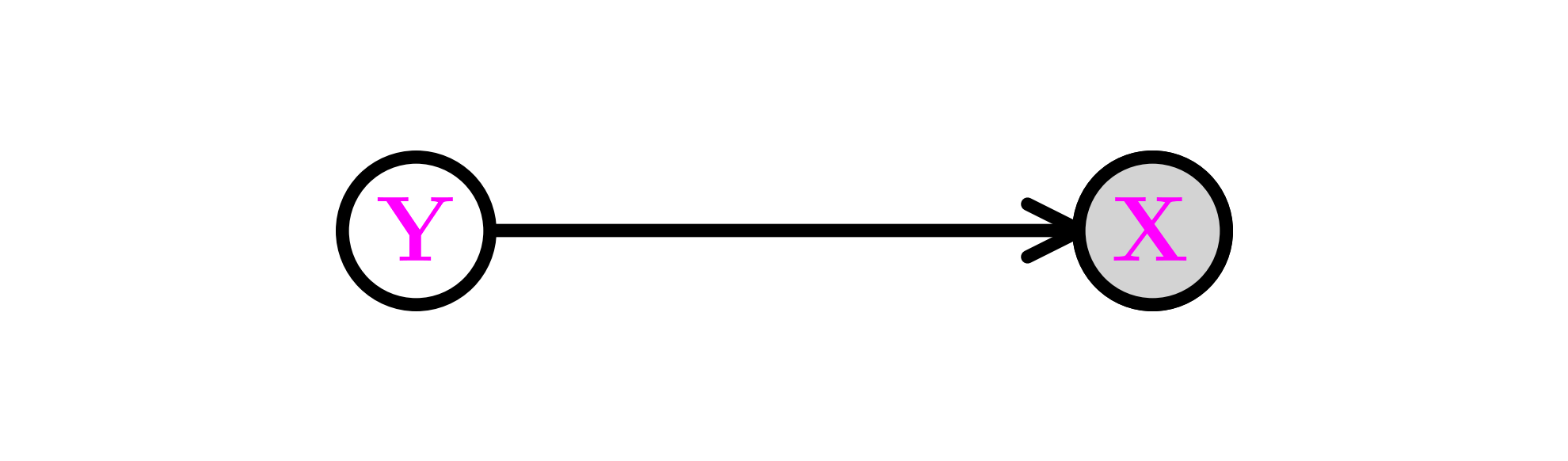
That can be represented in a digraph with a directed edge from a vertex for \(\mathbf{Y}\) to a vertex for \(\mathbf{X}\). Further, we let the vertex for \(\mathbf{X}\) be shaded to indicate that it is observed, while the vertex for \(\mathbf{Y}\) is not shaded to indicate that it is not. Mathematically, that corresponds to applying the law of total probability as we did previously.
In the parametric context, this gives rise to a fruitful approach to expanding distribution families. Suppose \(\{p_{\btheta}:\btheta \in \Theta\}\) is a parametric family of distributions. Let \(K \geq 2\), \(\btheta_1, \ldots, \btheta_K \in \Theta\) and \(\bpi = (\pi_1,\ldots,\pi_K) \in \Delta_K\). Suppose \(Y \sim \mathrm{Cat}(\bpi)\) and that the conditional distributions satisfy
We write this as \(\bX|\{Y=i\} \sim p_{\btheta_i}\). Then we obtain the mixture model
EXAMPLE: (Mixture of Multinomials) Let \(n, m , K \geq 1\), \(\bpi \in \Delta_K\) and, for \(i=1,\ldots,K\), \(\mathbf{p}_i = (p_{i1},\ldots,p_{im}) \in \Delta_m\). Suppose that \(Y \sim \mathrm{Cat}(\bpi)\) and that the conditional distributions are
Then \(\bX\) is a mixture of multinomials. Its distribution is then
\(\lhd\)
Next is an important continuous example.
EXAMPLE: (Gaussian mixture model) \(\idx{Gaussian mixture model}\xdi\) For \(i=1,\ldots,K\), let \(\bmu_i\) and \(\bSigma_i\) be the mean and covariance matrix of a multivariate Gaussian. Let \(\bpi \in \Delta_K\). A Gaussian Mixture Model (GMM) is obtained as follows: take \(Y \sim \mathrm{Cat}(\bpi)\) and
Its probability density function (PDF) takes the form
\(\lhd\)
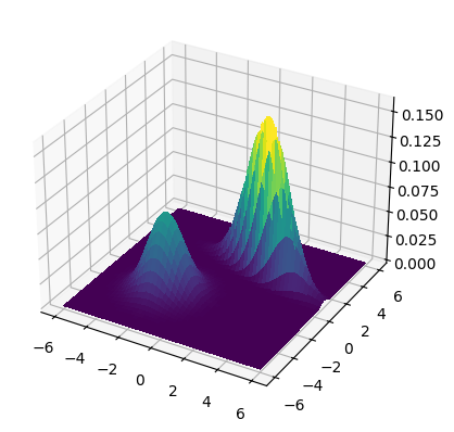
NUMERICAL CORNER: We plot the density for means \(\bmu_1 = (-2,-2)\) and \(\bmu_2 = (2,2)\) and covariance matrices
where \(\sigma_1 = 1.5\), \(\sigma_2 = 0.5\) and \(\rho = -0.75\). The mixing weights are \(\pi_1 = 0.25\) and \(\pi_2 = 0.75\).
from scipy.stats import multivariate_normal

def gmm2_pdf(X, Y, mean1, cov1, pi1, mean2, cov2, pi2):
    xy = np.stack([X.flatten(), Y.flatten()], axis=-1)
    Z1 = multivariate_normal.pdf(
        xy, mean=mean1, cov=cov1).reshape(X.shape)
    Z2 = multivariate_normal.pdf(
        xy, mean=mean2, cov=cov2).reshape(X.shape)
    return pi1 * Z1 + pi2 * Z2
Show code cell source
start_point = 6
stop_point = 6
num_samples = 100
points = np.linspace(-start_point, stop_point, num_samples)
X, Y = np.meshgrid(points, points)

mean1 = np.array([-2., -2.])
cov1 = np.array([[1., 0.], [0., 1.]])
pi1 = 0.5
mean2 = np.array([2., 2.])
cov2 = np.array([[1.5 ** 2., -0.75 * 1.5 * 0.5],
                 [-0.75 * 1.5 * 0.5, 0.5 ** 2.]])
pi2 = 0.5
Z = gmm2_pdf(X, Y, mean1, cov1, pi1, mean2, cov2, pi2)
mmids.make_surface_plot(X, Y, Z)
\(\unlhd\)
In NumPy, as we have seen before, the module numpy.random also provides a way to sample from mixture models by using numpy.random.Generator.choice.
For instance, we consider mixtures of multivariate Gaussians. We chage the notation slightly to track Python’s indexing. For \(i=0,1\), we have a mean \(\bmu_i \in \mathbb{R}^d\) and a positive definite covariance matrix \(\bSigma_i \in \mathbb{R}^{d \times d}\). We also have mixture weights \(\phi_0, \phi_1 \in (0,1)\) such that \(\phi_0 + \phi_1 = 1\). Suppose we want to generate a total of \(n\) samples.
For each sample \(j=1,\ldots, n\), independently from everything else:
We first pick a component \(i \in \{0,1\}\) at random according to the mixture weights, that is, \(i=0\) is chosen with probability \(\phi_0\) and \(i=1\) is chosen with probability \(\phi_1\).
We generate a sample \(\bX_j = (X_{j,1},\ldots,X_{j,d})\) according to a multivariate Gaussian with mean \(\bmu_i\) and covariance \(\bSigma_i\).
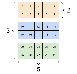
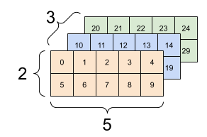
This is straightforward to implement by using again numpy.random.Generator.choice to choose the component of each sample and numpy.random.Generator.multivariate_normal to generate multivariate Gaussians. For convenience, we will stack the means and covariances into one array with a new dimension. So, for instance, the covariance matrices will now be in a 3d-array, that is, an array with \(3\) indices. The first index corresponds to the component (here \(0\) or \(1\)).
Figure: Three matrices (Source)
\(\bowtie\)
Figure: Three matrices stacked into a 3d-array (Source)
\(\bowtie\)
The code is the following. It returns an d by n array X, where each row is a sample from a 2-component Gaussian mixture.
def gmm2(rng, d, n, phi0, phi1, mu0, sigma0, mu1, sigma1):

    phi = np.stack((phi0, phi1))
    mu = np.stack((mu0, mu1))
    sigma = np.stack((sigma0,sigma1))

    X = np.zeros((n,d))
    component = rng.choice(2, size=n, p=phi)
    for i in range(n):
        X[i,:] = rng.multivariate_normal(
            mu[component[i],:],
            sigma[component[i],:,:])

    return X
NUMERICAL CORNER: Let us try it with following parameters. We first define the covariance matrices and show what happens when they are stacked into a 3d array (as is done within gmm2).
d = 2
sigma0 = np.outer(np.array([2., 2.]), np.array([2., 2.]))
sigma0 += np.outer(np.array([-0.5, 0.5]), np.array([-0.5, 0.5]))
sigma1 = 2 * np.identity(d)
sigma = np.stack((sigma0,sigma1))
print(sigma[0,:,:])
[[4.25 3.75]
 [3.75 4.25]]
print(sigma[1,:,:])
[[2. 0.]
 [0. 2.]]
Then we define the rest of the parameters.
seed = 535
rng = np.random.default_rng(seed)

n, w = 200, 5.
phi0 = 0.8
phi1 = 0.2
mu0 = np.concatenate(([w], np.zeros(d-1)))
mu1 = np.concatenate(([-w], np.zeros(d-1)))
X = gmm2(rng, d, n, phi0, phi1, mu0, sigma0, mu1, sigma1)

plt.scatter(X[:,0], X[:,1], s=5, marker='o', c='k')
plt.axis('equal')
plt.show()
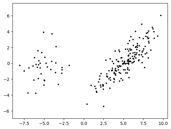
\(\unlhd\)
6.4.2. Example: Mixtures of multivariate Bernoullis and the EM algorithm#
Let \(\mathcal{C} = \{1, \ldots, K\}\) be a collection of classes. Let \(C\) be a random variable taking values in \(\mathcal{C}\) and, for \(m=1, \ldots, M\), let \(X_i\) take values in \(\{0,1\}\). Define \(\pi_k = \P[C = k]\) and \(p_{k,m} = \P[X_m = 1|C = k]\) for \(m = 1,\ldots, M\). We denote by \(\bX = (X_1, \ldots, X_M)\) the corresponding vector of \(X_i\)’s and assume that the entries are conditionally independent given \(C\).
However, we assume this time that \(C\) itself is not observed. So the resulting joint distribution is the mixture
Graphically, this is the same are the Naive Bayes model, except that \(C\) is not observed and therefore is not shaded.
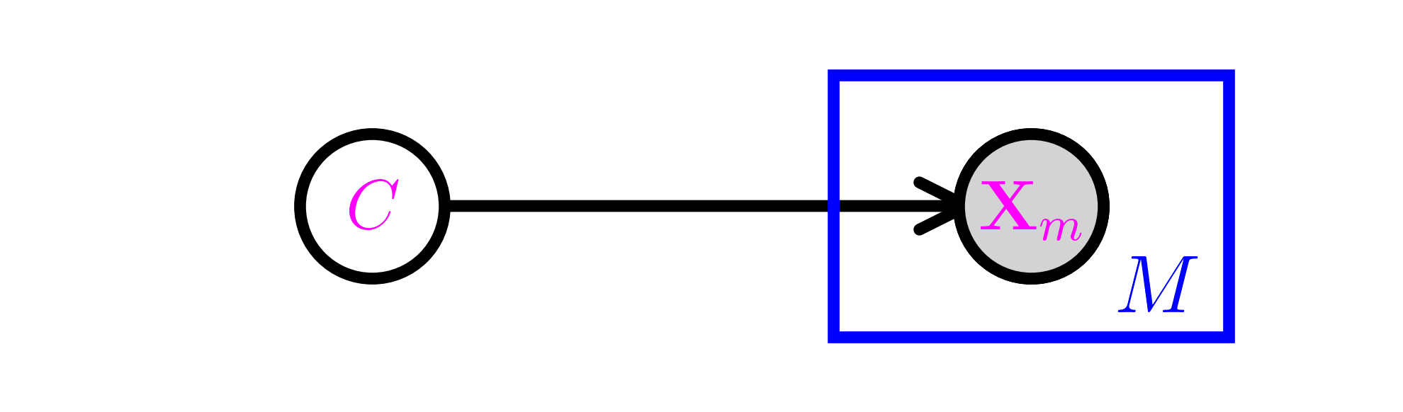
This type of model is useful in particular for clustering tasks, where the \(c_k\)s can be thought of as different clusters. Similarly to what we did in the previous section, our goal is to infer the parameters from samples and then predict the class of an old or new sample given its features. The main – substantial – difference is that the true labels of the samples are not observed. As we will see, that complicates the task considerably.
Model fitting We first fit the model from training data \(\{\bx_i\}_{i=1}^n\). Recall that the corresponding class labels \(c_i\)s are not observed. In this type of model, they are referred to as hidden or latent variables and we will come back to their inference below.
We would like to use maximum likelihood estimation, that is, maximize the probability of observing the data
As usual, we assume that the samples are independent and identically distributed. Consider the negative log-likelihood (NLL)
Already, we see that things are potentially more difficult than they were in the supervised (or fully observed) case. The NLL does not decompose into a sum of terms depending on different sets of parameters.
At this point, one could fall back on the field of optimization and use a gradient-based method to minimize the NLL. Indeed that is an option, although note that one must be careful to account for the constrained nature of the problem (i.e., the parameters sum to one). There is a vast array of constrained optimization techniques suited for this task.
Instead a more popular approach in this context, the EM algorithm, is based on the general principle of majorization-minimization, which we have encountered implicitly in the \(k\)-means algorithm and the convergence proof of gradient descent in the smooth case. We detail this important principle in the next subsection before returning to model fitting in mixtures.
Majorization-minimization \(\idx{majorization-minimization}\xdi\) Here is a deceptively simple, yet powerful observation. Suppose we want to minimize a function \(f : \mathbb{R}^d \to \mathbb{R}\). Finding a local minimum of \(f\) may not be easy. But imagine that for each \(\mathbf{x} \in \mathbb{R}^d\) we have a surrogate function \(U_{\mathbf{x}} : \mathbb{R}^d \to \mathbb{R}\) that (1) dominates \(f\) in the following sense
and (2) equals \(f\) at \(\mathbf{x}\)
We say that \(U_\mathbf{x}\) majorizes \(f\) at \(\mathbf{x}\). Then we prove in the next lemma that \(U_\mathbf{x}\) can be used to make progress towards minimizing \(f\), that is, find a point \(\mathbf{x}'\) such that \(f(\mathbf{x}') \leq f(\mathbf{x})\). If in addition \(U_\mathbf{x}\) is easier to minimize than \(f\) itself, say because an explicit minimum can be computed, then this observation naturally leads to an iterative algorithm.
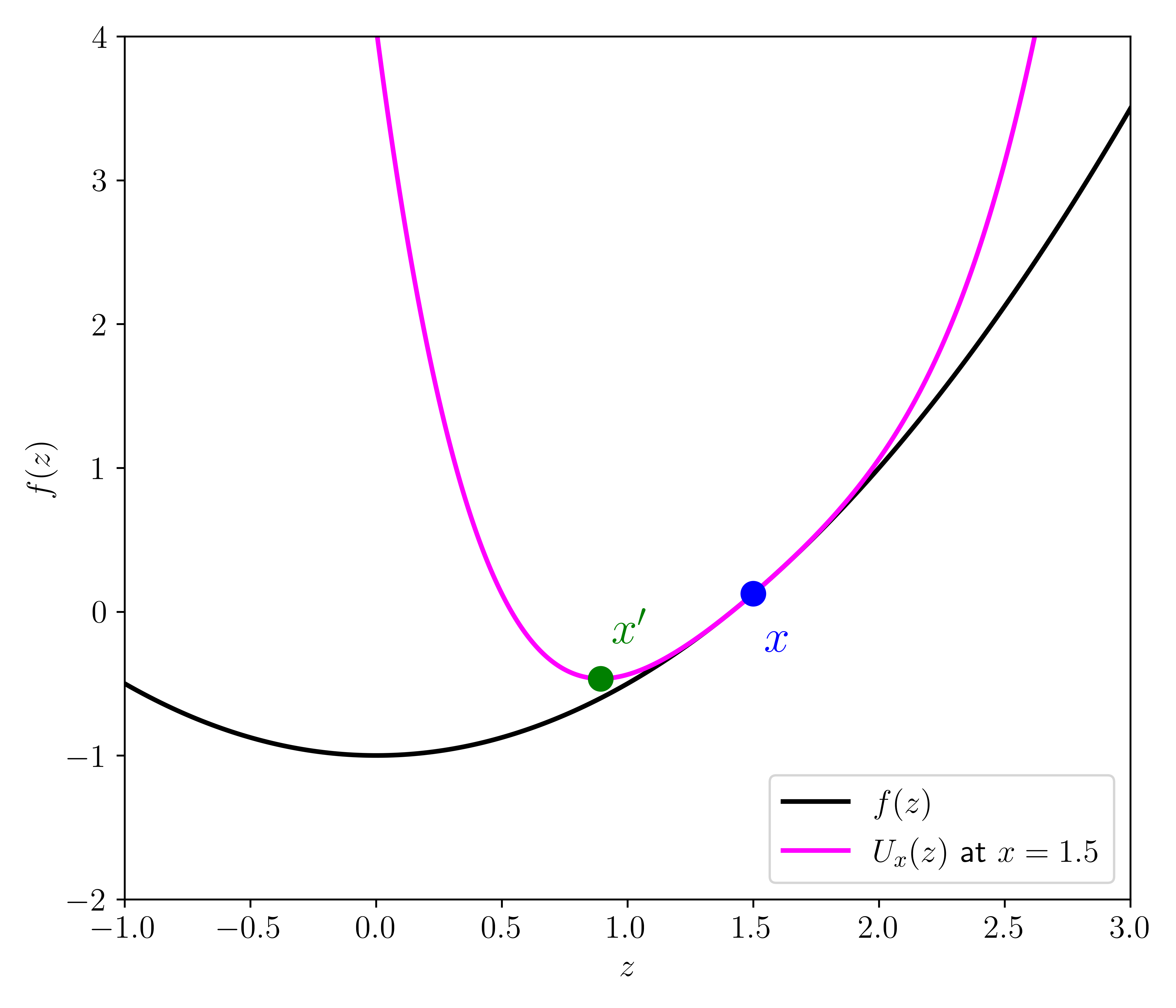
LEMMA (Majorization-Minimization) \(\idx{majorization-minimization lemma}\xdi\) Let \(f : \mathbb{R}^d \to \mathbb{R}\) and suppose \(U_{\mathbf{x}}\) majorizes \(f\) at \(\mathbf{x}\). Let \(\mathbf{x}'\) be a global minimum of \(U_\mathbf{x}\). Then
\(\flat\)
Proof: Indeed
where the first inequality follows from the domination property of \(U_\mathbf{x}\), the second inequality follows from the fact that \(\mathbf{x}'\) is a global minimum of \(U_\mathbf{x}\) and the equality follows from the fact that \(U_{\mathbf{x}}\) equals \(f\) at \(\mathbf{x}\). \(\square\)
We have already encountered this idea.
EXAMPLE: (Minimizing a smooth function) Let \(f : \mathbb{R}^d \to \mathbb{R}\) be \(L\)-smooth. By the Quadratic Bound for Smooth Functions, for all \(\mathbf{x}, \mathbf{z} \in \mathbb{R}^d\) it holds that
By showing that \(U_{\mathbf{x}}\) is minimized at \(\mathbf{z} = \mathbf{x} - (1/L)\nabla f(\mathbf{x})\), we previously obtained the descent guarantee
for gradient descent, which played a central role in the analysis of its convergence\(\idx{convergence analysis}\xdi\). \(\lhd\)
EXAMPLE: (\(k\)-means) \(\idx{Lloyd's algorithm}\xdi\) Let \(\mathbf{x}_1,\ldots,\mathbf{x}_n\) be \(n\) vectors in \(\mathbb{R}^d\). One way to formulate the \(k\)-means clustering problem is as the minimization of
over the centers \(\bmu_1,\ldots,\bmu_K\), where recall that \([K] = \{1,\ldots,K\}\). For fixed \(\bmu_1,\ldots,\bmu_K\) and \(\mathbf{m} = (\bmu_1,\ldots,\bmu_K)\), define
and
for \(\blambda_1,\ldots,\blambda_K \in \mathbb{R}^d\). That is, we fix the optimal cluster assignments under \(\bmu_1,\ldots,\bmu_K\) and then vary the centers.
We claim that \(U_\mathbf{m}\) is majorizing \(f\) at \(\bmu_1,\ldots,\bmu_K\). Indeed
and
Moreover \(U_\mathbf{m}(\blambda_1,\ldots,\blambda_K)\) is easy to minimize. We showed previously that the optimal representatives are
where \(C_j = \{i : c_\mathbf{m}(i) = j\}\).
The Majorization-Minimization Lemma implies that
This argument is equivalent to our previous analysis of the \(k\)-means algorithm. \(\lhd\)
CHAT & LEARN The mixture of multivariate Bernoullis model assumes a fixed number of clusters. Ask your favorite AI chatbot to discuss Bayesian nonparametric extensions of this model, such as the Dirichlet process mixture model, which can automatically infer the number of clusters from the data. \(\ddagger\)
EM algorithm The Expectation-Maximization (EM) algorithm\(\idx{EM algorithm}\xdi\) is an instantiation of the majorization-minimization principle that applies widely to parameter estimation of mixtures. Here we focus on the mixture of multivariate Bernoullis.
Recall that the objective to be minimized is
To simplify the notation and highlight the general idea, we let \(\btheta = (\bpi, \{\bp_k\})\), denote by \(\Theta\) the set of allowed values for \(\btheta\), and use \(\P_{\btheta}\) to indicate that probabilities are computed under the parameters \(\btheta\). We also return to the description of the model in terms of the unobserved latent variables \(\{C_i\}\). That is, we write the NLL as
To derive a majorizing function, we use the convexity of the negative logarithm. Indeed
The first step of the construction is not obvious – it just works. For each \(i=1,\ldots,n\), we let \(r_{k,i}^{\btheta}\), \(k=1,\ldots,K\), be a strictly positive probability distribution over \([K]\). In other words, it defines a convex combination for every \(i\). Then we use convexity to obtain the upper bound
which holds for any \(\tilde\btheta = (\tilde\bpi, \{\tilde\bp_k\}) \in \Theta\).
We choose
(which for the time being we assume is strictly positive) and we denote the right-hand side of the inequality by \(Q_{n}(\tilde\btheta|\btheta)\) (as a function of \(\tilde\btheta\)).
We make two observations.
1- Dominating property: For any \(\tilde\btheta \in \Theta\), the inequality above implies immediately that \(L_n(\tilde\btheta) \leq Q_n(\tilde\btheta|\btheta)\).
2- Equality at \(\btheta\): At \(\tilde\btheta = \btheta\),
The two properties above show that \(Q_n(\tilde\btheta|\btheta)\), as a function of \(\tilde\btheta\), majorizes \(L_n\) at \(\btheta\).
LEMMA (EM Guarantee) \(\idx{EM guarantee}\xdi\) Let \(\btheta^*\) be a global minimizer of \(Q_n(\tilde\btheta|\btheta)\) as a function of \(\tilde\btheta\), provided it exists. Then
\(\flat\)
Proof: The result follows directly from the Majorization-Minimization Lemma. \(\square\)
What have we gained from this? As we mentioned before, using the Majorization-Minimization Lemma makes sense if \(Q_n\) is easier to minimize than \(L_n\) itself. Let us see why that is the case here.
E Step: The function \(Q_n\) naturally decomposes into two terms
Because \(r_{k,i}^{\btheta}\) depends on \(\btheta\) but not \(\tilde\btheta\), the second term is irrelevant to the opimization with respect to \(\tilde\btheta\).
The first term above can be written as
where we defined, for \(k=1,\ldots,K\),
Here comes the key observation: this last expression is essentially the same as the NLL for the fully observed Naive Bayes model, except that the terms \(\mathbf{1}_{\{c_i = k\}}\) are replaced by \(r_{k,i}^{\btheta}\). If \(\btheta\) is our current estimate of the parameters, then the quantity \(r_{k,i}^{\btheta} = \P_{\btheta}[C_i = k|\bX_i = \bx_i]\) is our estimate – under the current parameter \(\btheta\) – of the probability that the sample \(\bx_i\) comes from cluster \(k\). We have previously computed \(r_{k,i}^{\btheta}\) for prediction under the Naive Bayes model. We showed there that
which in this new context is referred to as the responsibility that cluster \(k\) takes for data point \(i\). So we can interpret the expression above as follows: the variables \(\mathbf{1}_{\{c_i = k\}}\) are not observed here, but we have estimated their conditional probability distribution given the observed data \(\{\bx_i\}\), and we are taking an expectation with respect to that distribution instead.
The “E” in E Step (and EM) stands for “expectation”, which refers to using a surrogate function that is essentially an expected NLL.
M Step: In any case, from a practical point of view, minimizing \(Q_n(\tilde\btheta|\btheta)\) over \(\tilde\btheta\) turns out to be a variant of fitting a Naive Bayes model – and the upshot to all this is that there is a straightforward formula for that! Recall that this happens because, the NLL in the Naive Bayes model decomposes: it naturally breaks up into terms that depend on separate sets of parameters, each of which can be optimized with a closed-form expression. The same happens with \(Q_n\) as should be clear from the derivation.
Adapting our previous calculations for fitting a Naive Bayes model, we get that \(Q_n(\tilde\btheta|\btheta)\) is minimized at
We used the fact that
since the conditional probability \(\P_{\btheta}[C_i = k|\bX_i = \bx_i]\) adds up to one when summed over \(k\).
The “M” in M Step (and EM) stands for maximization, which here turns into minimization because of the use of the NLL.
To summarize, the EM algorithm works as follows in this case. Assume we have data points \(\{\bx_i\}_{i=1}^n\), that we have fixed \(K\) and that we have some initial parameter estimate \(\btheta^0 = (\bpi^0, \{\bp_k^0\}) \in \Theta\) with strictly positive \(\pi_k^0\)s and \(p_{k,m}^0\)s. For \(t = 0,1,\ldots, T-1\) we compute for all \(i \in [n]\), \(k \in [K]\), and \(m \in [M]\)
and
Provided \(\sum_{i=1}^n x_{i,m} > 0\) for all \(m\), the \(\eta_{k,m}^t\)s and \(\eta_k^t\)s remain positive for all \(t\) and the algorithm is well-defined. The EM Guarantee stipulates that the NLL cannot deteriorate, although note that it does not guarantee convergence to a global minimum.
We implement the EM algorithm for mixtures of multivariate Bernoullis. For this purpose, we adapt our previous Naive Bayes routines. We also allow for the possibility of using Laplace smoothing.
def responsibility(pi_k, p_km, x):

    K = len(pi_k)
    score_k = np.zeros(K)
    for k in range(K):

        score_k[k] -= np.log(pi_k[k])
        score_k[k] -= np.sum(x * np.log(p_km[k,:])
                             + (1 - x) * np.log(1 - p_km[k,:]))
    r_k = np.exp(-score_k)/(np.sum(np.exp(-score_k)))

    return r_k

def update_parameters(eta_km, eta_k, eta, alpha, beta):

    K = len(eta_k)
    pi_k = (eta_k+alpha) / (eta+K*alpha)
    p_km = (eta_km+beta) / (eta_k[:,np.newaxis]+2*beta)

    return pi_k, p_km
We implement the E and M Step next.
def em_bern(X, K, pi_0, p_0, maxiters = 10, alpha=0., beta=0.):

    n, M = X.shape
    pi_k = pi_0
    p_km = p_0

    for _ in range(maxiters):

        # E Step
        r_ki = np.zeros((K,n))
        for i in range(n):
            r_ki[:,i] = responsibility(pi_k, p_km, X[i,:])

        # M Step
        eta_km = np.zeros((K,M))
        eta_k = np.sum(r_ki, axis=-1)
        eta = np.sum(eta_k)
        for k in range(K):
            for m in range(M):
                eta_km[k,m] = np.sum(X[:,m] * r_ki[k,:])
        pi_k, p_km = update_parameters(
            eta_km, eta_k, eta, alpha, beta)

    return pi_k, p_km
NUMERICAL CORNER: We test the algorithm on a very simple dataset.
X = np.array([[1., 1., 1.],[1., 1., 1.],[1., 1., 1.],[1., 0., 1.],
              [0., 1., 1.],[0., 0., 0.],[0., 0., 0.],[0., 0., 1.]])
n, M = X.shape
K = 2
pi_0 = np.ones(K)/K
p_0 = rng.random((K,M))

pi_k, p_km = em_bern(
    X, K, pi_0, p_0, maxiters=100, alpha=0.01, beta=0.01)

print(pi_k)
[0.66500949 0.33499051]
print(p_km)
[[0.74982646 0.74982646 0.99800266]
 [0.00496739 0.00496739 0.25487292]]
We compute the probability that the vector \((0, 0, 1)\) is in each cluster.
x_test = np.array([0., 0., 1.])
print(responsibility(pi_k, p_km, x_test))
[0.32947702 0.67052298]
CHAT & LEARN The EM algorithm can sometimes get stuck in local optima. Ask your favorite AI chatbot to discuss strategies for initializing the EM algorithm to avoid this issue, such as using multiple random restarts or using the k-means algorithm for initialization. (Open In Colab) \(\ddagger\)
\(\unlhd\)
6.4.3. Clustering handwritten digits#
To give a more involved example, we use the MNIST dataset.
Quoting Wikipedia again:
The MNIST database (Modified National Institute of Standards and Technology database) is a large database of handwritten digits that is commonly used for training various image processing systems. The database is also widely used for training and testing in the field of machine learning. It was created by “re-mixing” the samples from NIST’s original datasets. The creators felt that since NIST’s training dataset was taken from American Census Bureau employees, while the testing dataset was taken from American high school students, it was not well-suited for machine learning experiments. Furthermore, the black and white images from NIST were normalized to fit into a 28x28 pixel bounding box and anti-aliased, which introduced grayscale levels. The MNIST database contains 60,000 training images and 10,000 testing images. Half of the training set and half of the test set were taken from NIST’s training dataset, while the other half of the training set and the other half of the test set were taken from NIST’s testing dataset.
Figure: MNIST sample images (Source)

\(\bowtie\)
NUMERICAL CORNER: We load it from PyTorch. The data can be accessed with torchvision.datasets.MNIST. The squeeze() below removes the color dimension in the image, which is grayscale. The numpy() converts the PyTorch tensors into NumPy arrays. See torch.utils.data.DataLoader for details on the data loading. We will say more about PyTorch in a later chapter.
Show code cell source
from torchvision import datasets, transforms
from torch.utils.data import DataLoader

mnist = datasets.MNIST(root='./data', train=True,
                       download=True, transform=transforms.ToTensor())
train_loader = DataLoader(mnist, batch_size=len(mnist), shuffle=False)

imgs, labels = next(iter(train_loader))
imgs = imgs.squeeze().numpy()
labels = labels.numpy()
We turn the grayscale images into a black-and-white images by rounding the pixels.
imgs = np.round(imgs)
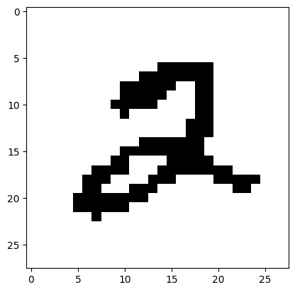
There are two common ways to write a \(2\). Let’s see if a mixture of multivariate Bernoullis can find them. We extract the images labelled \(2\).
mask = labels == 2
imgs2 = imgs[mask]
labels2 = labels[mask]
The first image is the following.
Show code cell source
plt.imshow(imgs2[0], cmap='gray_r')
plt.show()
Next, we transform the images into vectors.
X = imgs2.reshape(len(imgs2), -1)
We run the algorithm with \(2\) clusters.
n, M = X.shape
K = 2
pi_0 = np.ones(K)/K
p_0 = rng.random((K,M))

pi_k, p_km = em_bern(
    X, K, pi_0, p_0, maxiters=10, alpha=1., beta=1.)

print(pi_k)
[nan nan]
Uh-oh. Something went wrong. We encountered a numerical issue, underflow, which we discussed briefly previously. To confirm this, we run the code again but ask Python to warn us about it using numpy.seterr. (By default, warnings are turned off in the book, but they can be reactivated using warnings.resetwarnings.)
warnings.resetwarnings()
old_settings = np.seterr(all='warn')

pi_k, p_km = em_bern(
    X, K, pi_0, p_0, maxiters=10, alpha=1., beta=1.)
/var/folders/k0/7k0fxl7j54q4k8dyqnrc6sz00000gr/T/ipykernel_84428/861379570.py:10: RuntimeWarning: underflow encountered in exp
  r_k = np.exp(-score_k)/(np.sum(np.exp(-score_k)))
/var/folders/k0/7k0fxl7j54q4k8dyqnrc6sz00000gr/T/ipykernel_84428/861379570.py:10: RuntimeWarning: invalid value encountered in divide
  r_k = np.exp(-score_k)/(np.sum(np.exp(-score_k)))
\(\unlhd\)
When we compute the responsibilities
we first compute the negative logarithm of each term in the numerator as we did in the Naive Bayes case. But then we apply the function \(e^{-x}\), because this time we are not simply computing an optimal score. When all scores are high, this last step may result in underflow, that is, produces numbers so small that they get rounded down to zero by NumPy. Then the ratio defining r_k is not well-defined.
To deal with this, we introduce a technique called the log-sum-exp trick\(\idx{log-sum-exp trick}\xdi\) (with some help from ChatGPT). Consider the computation of a function of \(\mathbf{a} = (a_1, \ldots, a_n)\) of the form
When the \(a_i\) values are large positive numbers, the terms \(e^{-a_i}\) can be so small that they underflow to zero. To counter this, the log-sum-exp trick involves a shift to bring these terms into a more favorable numerical range.
It proceeds as follows:
Identify the minimum value \(M\) among the \(a_i\)s
\[ M = \min\{a_1, a_2, \ldots, a_n\}. \]Subtract \(M\) from each \(a_i\) before exponentiation
\[ \log \left( \sum_{i=1}^{n} e^{-a_i} \right) = \log \left( e^{-M} \sum_{i=1}^{n} e^{- (a_i - M)} \right). \]Rewrite using log properties
\[ = -M + \log \left( \sum_{i=1}^{n} e^{-(a_i - M)} \right). \]
Why does this help with underflow? By subtracting \(M\), the smallest value in the set, from each \(a_i\): (i) the largest term in \(\{e^{-(a_i - M)} : i = 1,\ldots,n\}\) becomes \(e^0 = 1\); and (ii) all other terms are between 0 and 1, as they are exponentiations of nonpositive numbers. This manipulation avoids terms underflowing to zero because even very large values, when shifted by \(M\), are less likely to hit the underflow threshold.
Here is an example. Imagine you have \(\mathbf{a} = (1000, 1001, 1002)\).
Direct computation: \(e^{-1000}\), \(e^{-1001}\), and \(e^{-1002}\) might all underflow to zero.
With the log-sum-exp trick: Subtract \(M = 1000\), leading to \(e^{0}\), \(e^{-1}\), and \(e^{-2}\), all meaningful, non-zero results that accurately contribute to the sum.
We implement in NumPy.
def log_sum_exp_trick(a):
    min_val = np.min(a)
    return - min_val + np.log(np.sum(np.exp(- a + min_val)))
NUMERICAL CORNER: We try it on a simple example.
a = np.array([1000, 1001, 1002])
We first attempt a direct computation.
np.log(np.sum(np.exp(-a)))
/var/folders/k0/7k0fxl7j54q4k8dyqnrc6sz00000gr/T/ipykernel_84428/214275762.py:1: RuntimeWarning: underflow encountered in exp
  np.log(np.sum(np.exp(-a)))
/var/folders/k0/7k0fxl7j54q4k8dyqnrc6sz00000gr/T/ipykernel_84428/214275762.py:1: RuntimeWarning: divide by zero encountered in log
  np.log(np.sum(np.exp(-a)))
-inf
Predictly, we get an underflow error and a useless output.
Next, we try the log-sum-exp trick.
log_sum_exp_trick(a)
-999.5923940355556
This time we get an output which seems reasonable, something slightly larger than \(-1000\) as expected (Why?).
\(\unlhd\)
After this long – but important! – parenthesis, we return to the EM algorithm. We modify it by implementing the log-sum-exp trick in the subroutine responsibility.
def responsibility(pi_k, p_km, x):

    K = len(pi_k)
    score_k = np.zeros(K)
    for k in range(K):

        score_k[k] -= np.log(pi_k[k])
        score_k[k] -= np.sum(x * np.log(p_km[k,:])
                             + (1 - x) * np.log(1 - p_km[k,:]))
    r_k = np.exp(-score_k - log_sum_exp_trick(score_k))

    return r_k
NUMERICAL CORNER: We go back to the MNIST example with only the 2s.
pi_k, p_km = em_bern(X, K, pi_0, p_0, maxiters=10, alpha=1., beta=1.)
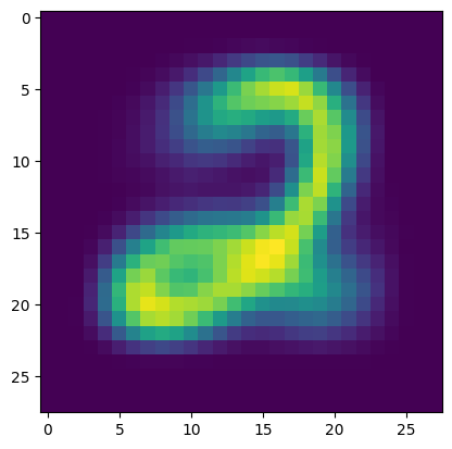
Here are the parameters for one cluster.
plt.figure()
plt.imshow(p_km[0,:].reshape((28,28)))
plt.show()
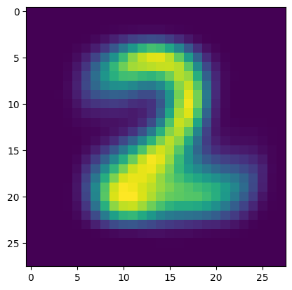
Here is the other one.
plt.figure()
plt.imshow(p_km[1,:].reshape((28,28)))
plt.show()
Now that the model is trained, we compute the probability that an example image is in each cluster. We use the first image in the dataset that we plotted earlier.
responsibility(pi_k, p_km, X[0,:])
array([1.00000000e+00, 5.09357087e-17])
It indeed identifies the second cluster as significantly more likely.
TRY IT! In the MNIST example, as we have seen, the probabilities involved are extremely small and the responsibilities are close to \(0\) or \(1\). Implement a variant of EM, called hard EM, which replaces responsibilities with the one-hot encoding of the largest responsibility. Test it on the MNIST example again. (Open In Colab)
\(\unlhd\)
CHAT & LEARN The mixture of multivariate Bernoullis model is a simple example of a latent variable model. Ask your favorite AI chatbot to discuss more complex latent variable models, such as the variational autoencoder or the Gaussian process latent variable model, and their applications in unsupervised learning. \(\ddagger\)
Self-assessment quiz (with help from Claude, Gemini, and ChatGPT)
1 In the mixture of multivariate Bernoullis model, the joint distribution is given by:
a) \(\mathbb{P}[\mathbf{X} = \mathbf{x}] = \prod_{k=1}^K \mathbb{P}[C = k, \mathbf{X} = \mathbf{x}]\)
b) \(\mathbb{P}[\mathbf{X} = \mathbf{x}] = \sum_{k=1}^K \mathbb{P}[\mathbf{X} = \mathbf{x}|C = k] \mathbb{P}[C = k]\)
c) \(\mathbb{P}[\mathbf{X} = \mathbf{x}] = \prod_{k=1}^K \mathbb{P}[\mathbf{X} = \mathbf{x}|C = k] \mathbb{P}[C = k]\)
d) \(\mathbb{P}[\mathbf{X} = \mathbf{x}] = \sum_{\mathbf{x}} \mathbb{P}[C = k, \mathbf{X} = \mathbf{x}]\)
2 The majorization-minimization principle states that:
a) If \(U_{\mathbf{x}}\) majorizes \(f\) at \(\mathbf{x}\), then a global minimum \(\mathbf{x}'\) of \(U_{\mathbf{x}}\) satisfies \(f(\mathbf{x}') \geq f(\mathbf{x})\).
b) If \(U_{\mathbf{x}}\) majorizes \(f\) at \(\mathbf{x}\), then a global minimum \(\mathbf{x}'\) of \(U_{\mathbf{x}}\) satisfies \(f(\mathbf{x}') \leq f(\mathbf{x})\).
c) If \(U_{\mathbf{x}}\) minorizes \(f\) at \(\mathbf{x}\), then a global minimum \(\mathbf{x}'\) of \(U_{\mathbf{x}}\) satisfies \(f(\mathbf{x}') \geq f(\mathbf{x})\).
d) If \(U_{\mathbf{x}}\) minorizes \(f\) at \(\mathbf{x}\), then a global minimum \(\mathbf{x}'\) of \(U_{\mathbf{x}}\) satisfies \(f(\mathbf{x}') \leq f(\mathbf{x})\).
3 In the EM algorithm for mixtures of multivariate Bernoullis, the M-step involves:
a) Updating the parameters \(\pi_k\) and \(p_{k,m}\)
b) Computing the responsibilities \(r_{k,i}^t\)
c) Minimizing the negative log-likelihood
d) Applying the log-sum-exp trick
4 The mixture of multivariate Bernoullis model is represented by the following graphical model:
a)
G = nx.DiGraph()
G.add_node("X", shape="circle", style="filled", fillcolor="gray")
G.add_node("C", shape="circle", style="filled", fillcolor="white")
G.add_edge("C", "X")
b)
G = nx.DiGraph()
G.add_node("X", shape="circle", style="filled", fillcolor="white")
G.add_node("C", shape="circle", style="filled", fillcolor="gray")
G.add_edge("C", "X")
c)
G = nx.DiGraph()
G.add_node("X", shape="circle", style="filled", fillcolor="gray")
G.add_node("C", shape="circle", style="filled", fillcolor="gray")
G.add_edge("C", "X")
d)
G = nx.DiGraph()
G.add_node("X", shape="circle", style="filled", fillcolor="white")
G.add_node("C", shape="circle", style="filled", fillcolor="white")
G.add_edge("C", "X")
5 In the context of clustering, what is the interpretation of the responsibilities computed in the E-step of the EM algorithm?
a) They represent the distance of each data point to the cluster centers.
b) They indicate the probability of each data point belonging to each cluster.
c) They determine the optimal number of clusters.
d) They are used to initialize the cluster centers in the M-step.
Answer for 1: b. Justification: The text states, “\(\mathbb{P}[\mathbf{X} = \mathbf{x}] = \sum_{k=1}^K \mathbb{P}[C = k, \mathbf{X} = \mathbf{x}] = \sum_{k=1}^K \mathbb{P}[\mathbf{X} = \mathbf{x}|C = k] \mathbb{P}[C = k]\).”
Answer for 2: b. Justification: “Let \(f: \mathbb{R}^d \to \mathbb{R}\) and suppose \(U_{\mathbf{x}}\) majorizes \(f\) at \(\mathbf{x}\). Let \(\mathbf{x}'\) be a global minimizer of \(U_{\mathbf{x}}(\mathbf{z})\) as a function of \(\mathbf{z}\), provided it exists. Then \(f(\mathbf{x}') \leq f(\mathbf{x})\).”
Answer for 3: a. Justification: In the summary of the EM algorithm, the M-step is described as updating the parameters: “\(\pi_k^{t+1} = \frac{\eta_k^t}{n}\) and \(p_{k,m}^{t+1} = \frac{\eta_{k,m}^t}{\eta_k^t}\),” which require the responsibilities.
Answer for 4: b. Justification: The text states, “Mathematically, that corresponds to applying the law of total probability as we did previously. Further, we let the vertex for \(X\) be shaded to indicate that it is observed, while the vertex for \(Y\) is not shaded to indicate that it is not.”
Answer for 5: b. Justification: The text refers to responsibilities as “our estimate – under the current parameter – of the probability that the sample comes from cluster \(k\).”