\(\newcommand{\bSigma}{\boldsymbol{\Sigma}}\) \(\newcommand{\bmu}{\boldsymbol{\mu}}\) \(\newcommand{\blambda}{\boldsymbol{\lambda}}\)
3.8. Online supplementary materials#
3.8.1. Quizzes, solutions, code, etc.#
3.8.1.1. Just the code#
An interactive Jupyter notebook featuring the code in this chapter can be accessed below (Google Colab recommended). You are encouraged to tinker with it. Some suggested computational exercises are scattered throughout. The notebook is also available as a slideshow.
3.8.1.2. Self-assessment quizzes#
A more extensive web version of the self-assessment quizzes is available by following the links below.
3.8.1.3. Auto-quizzes#
Automatically generated quizzes for this chapter can be accessed here (Google Colab recommended).
3.8.1.4. Solutions to odd-numbered warm-up exercises#
(with help from Claude, Gemini, and ChatGPT)
Answer and justification for E3.2.1:
At the point \((1, -1)\), we have:
Answer and justification for E3.2.3:
At the point \((\frac{\pi}{4}, \frac{\pi}{3})\), we have:
Answer and justification for E3.2.5: The Hessian matrix of \(f(x_1, x_2)\) is:
At the point \((1, 2)\), we have:
We can see that \(\frac{\partial^2 f}{\partial x_1 \partial x_2}(1, 2) = \frac{\partial^2 f}{\partial x_2 \partial x_1}(1, 2) = 12\), confirming the Symmetry of the Hessian Theorem.
Answer and justification for E3.2.7:
Answer and justification for E3.2.9: The Hessian matrix is given by:
Answer and justification for E3.2.11: \(\frac{\partial f}{\partial x} = 3x^2y^2 - 2y^3\) and \(\frac{\partial f}{\partial y} = 2x^3y - 6xy^2 + 4y^3\), obtained by differentiating \(f\) with respect to each variable while holding the other constant.
Answer and justification for E3.2.13: The Hessian matrix is given by
Answer and justification for E3.2.15: \(\frac{\partial^2 q}{\partial x^2} = 6x\) and \(\frac{\partial^2 q}{\partial y^2} = -6x\). Adding these gives \(6x - 6x = 0\), so \(q\) satisfies Laplace’s equation.
Answer and justification for E3.2.17: By the chain rule, the rate of change of temperature experienced by the particle is
We have \(\nabla u(x, y) = (-2xe^{-x^2 - y^2}, -2ye^{-x^2 - y^2})\) and \(\mathbf{c}'(t) = (2t, 3t^2)\). Evaluating at \(t = 1\) gives
Answer and justification for E3.2.19: \(\frac{d}{dt} f(\mathbf{g}(t)) = 2t \cos t - t^2 \sin t\). Justification: \(\nabla f = (y, x)\), and \(\mathbf{g}'(t) = (2t, -\sin t)\). Then, \(\frac{d}{dt} f(\mathbf{g}(t)) = \cos t \cdot 2t + t^2 \cdot (-\sin t)\).
Answer and justification for E3.3.1: \(\nabla f(x_1, x_2) = (2x_1, 4x_2)\). Setting this equal to zero yields \(2x_1 = 0\) and \(4x_2 = 0\), which implies \(x_1 = 0\) and \(x_2 = 0\). Thus, the only point where \(\nabla f(x_1, x_2) = 0\) is \((0, 0)\).
Answer and justification for E3.3.3: The second directional derivative is given by \(\frac{\partial^2 f(\mathbf{x}_0)}{\partial \mathbf{v}^2} = \mathbf{v}^T \mathbf{H}_f(\mathbf{x}_0) \mathbf{v}\). We have \(\mathbf{H}_f(x_1, x_2) = \begin{pmatrix} 2 & 2 \\ 2 & 2 \end{pmatrix}\). Thus,
Answer and justification for E3.3.5: The first-order necessary conditions are:
Computing the gradients:
From the first two equations, we have \(x_1 = x_2 = -\frac{\lambda}{2}\). Substituting into the third equation:
Thus, \(x_1 = x_2 = \frac{1}{2}\), and the only point satisfying the first-order necessary conditions is \((\frac{1}{2}, \frac{1}{2}, -1)\).
Answer and justification for E3.3.7: The Lagrangian is \(L(x_1, x_2, x_3, \lambda) = x_1^2 + x_2^2 + x_3^2 + \lambda(x_1 + 2x_2 + 3x_3 - 6)\). The first-order necessary conditions are:
From the first three equations, we have \(x_1 = -\frac{\lambda}{2}\), \(x_2 = -\lambda\), \(x_3 = -\frac{3\lambda}{2}\). Substituting into the fourth equation:
Thus, \(x_1 = \frac{1}{2}\), \(x_2 = 1\), \(x_3 = \frac{3}{2}\), and the only point satisfying the first-order necessary conditions is \((\frac{1}{2}, 1, \frac{3}{2}, -1)\).
Answer and justification for E3.3.9: The gradient of \(f\) is \(\nabla f(x_1, x_2) = (3x_1^2 - 3x_2^2, -6x_1x_2)\). At the point \((1, 0)\), the gradient is \(\nabla f(1, 0) = (3, 0)\). The directional derivative of \(f\) at \((1, 0)\) in the direction \(\mathbf{v} = (1, 1)\) is \(\nabla f(1, 0)^T \mathbf{v} = (3, 0)^T (1, 1) = 3\). Since this is positive, \(v\) is not a descent direction.
Answer and justification for E3.3.11: The Hessian matrix of \(f\) is
Therefore, the second directional derivative of \(f\) at \((0, 0)\) in the direction \(v = (1, 0)\) is \(\mathbf{v}^T \mathbf{H}_f(0, 0) \mathbf{v} = (1, 0) \begin{bmatrix} -2 & 0 \\ 0 & -2 \end{bmatrix} \begin{pmatrix} 1 \\ 0 \end{pmatrix} = -2\).
Answer and justification for E3.3.13: The Hessian matrix is
Justification: Compute the second partial derivatives:
At \((1,1)\), these values are \(6\), \(6\), and \(-3\), respectively.
Answer and justification for E3.4.1: The convex combination is:
Answer and justification for E3.4.3: \(S_1\) and \(S_2\) are halfspaces, which are convex sets. By the lemma in the text, the intersection of convex sets is also convex. Therefore, \(S_1 \cap S_2\) is a convex set.
Answer and justification for E3.4.5: The function \(f\) is a quadratic function with \(P = 2\), \(q = 2\), and \(r = 1\). Since \(P > 0\), \(f\) is strictly convex. The unique global minimizer is found by setting the gradient to zero:
Answer and justification for E3.4.7: The Hessian matrix of \(f\) is:
For any \((x, y) \in \mathbb{R}^2\), we have:
so \(f\) is strongly convex with \(m = 2\).
Answer and justification for E3.4.9: \(f\) is not convex. We have \(f''(x) = 12x^2 - 4\), which is negative for \(x \in (-\frac{1}{\sqrt{3}}, \frac{1}{\sqrt{3}})\). Since the second derivative is not always nonnegative, \(f\) is not convex.
Answer and justification for E3.4.11: \(f\) is strongly convex. We have \(f''(x) = 2 > 0\), so \(f\) is 2-strongly convex.
Answer and justification for E3.4.13: \(D\) is convex. To show this, let \((x_1, y_1), (x_2, y_2) \in D\) and \(\alpha \in (0, 1)\). We need to show that \((1 - \alpha)(x_1, y_1) + \alpha(x_2, y_2) \in D\). Compute:
Now,
Hence, \(D\) is convex.
Answer and justification for E3.4.15: \(D\) is not convex. For example, let \((x_1, y_1) = (2, \sqrt{3})\) and \((x_2, y_2) = (2, -\sqrt{3})\), both of which are in \(D\). For \(\alpha = \frac{1}{2}\),
Now,
Answer and justification for E3.5.1: The gradient is \(\nabla f(x, y) = (2x, 8y)\). At \((1, 1)\), it is \((2, 8)\). The direction of steepest descent is \(-\nabla f(1, 1) = (-2, -8)\).
Answer and justification for E3.5.3: \(\nabla f(x) = 3x^2 - 12x + 9\). At \(x_0 = 0\), \(\nabla f(0) = 9\). The first iteration gives \(x_1 = x_0 - \alpha \nabla f(x_0) = 0 - 0.1 \cdot 9 = -0.9\). At \(x_1 = -0.9\), \(\nabla f(-0.9) = 3 \cdot (-0.9)^2 - 12 \cdot (-0.9) + 9 = 2.43 + 10.8 + 9 = 22.23\). The second iteration gives \(x_2 = x_1 - \alpha \nabla f(x_1) = -0.9 - 0.1 \cdot 22.23 = -3.123\).
Answer and justification for E3.5.5: We have \(\nabla f(x) = 2x\), so \(\nabla f(2) = 4\). Thus, the gradient descent update is \(x_1 = x_0 - \alpha \nabla f(x_0) = 2 - 0.1 \cdot 4 = 1.6\).
Answer and justification for E3.5.7: \(f''(x) = 4\) for all \(x \in \mathbb{R}\). Therefore, \(f''(x) \geq 4\) for all \(x \in \mathbb{R}\), which implies that \(f\) is \(4\)-strongly convex.
Answer and justification for E3.5.9: No. We have \(f''(x) = 12x^2\), which can be arbitrarily large as \(x\) increases. Thus, there is no constant \(L\) such that \(-L \le f''(x) \le L\) for all \(x \in \mathbb{R}\).
Answer and justification for E3.5.11: We have \(f''(x) = 2\) for all \(x \in \mathbb{R}\). Thus, we can take \(m = 2\), and we have \(f''(x) \ge 2\) for all \(x \in \mathbb{R}\), which is the condition for \(m\)-strong convexity.
Answer and justification for E3.5.13: The gradient is \(\nabla f(x, y) = (2x, 2y)\). At \((1, 1)\), it is \((2, 2)\). The first update is \((0.8, 0.8)\). The gradient at \((0.8, 0.8)\) is \((1.6, 1.6)\). The second update is \((0.64, 0.64)\).
Answer and justification for E3.6.1: The log-odds is given by \(\log \frac{p}{1-p} = \log \frac{0.25}{0.75} = \log \frac{1}{3} = -\log 3\).
Answer and justification for E3.6.3:
Answer and justification for E3.6.5: By the quotient rule,
Answer and justification for E3.6.7: We have \(b_1 - \sigma(\boldsymbol{\alpha}_1^T \mathbf{x}) \approx 0.05\), \(b_2 - \sigma(\boldsymbol{\alpha}_2^T \mathbf{x}) \approx -0.73\), \(b_3 - \sigma(\boldsymbol{\alpha}_3^T \mathbf{x}) \approx 0.73\). Therefore,
Answer and justification for E3.6.9: We have \(b_1 - \sigma(\boldsymbol{\alpha}_1^T \mathbf{x}^0) = 1 - \sigma(0) = 0.5\), \(b_2 - \sigma(\boldsymbol{\alpha}_2^T \mathbf{x}^0) = -0.5\), \(b_3 - \sigma(\boldsymbol{\alpha}_3^T \mathbf{x}^0) = 0.5\). Therefore,
3.8.1.5. Learning outcomes#
Define and calculate partial derivatives and gradients for functions of several variables.
Compute second-order partial derivatives and construct the Hessian matrix for twice continuously differentiable functions.
Apply the Chain Rule to compute derivatives of composite functions of several variables.
State and prove the multivariable version of the Mean Value Theorem using the Chain Rule.
Calculate gradients and Hessians for affine and quadratic functions of several variables.
Define global and local minimizers for unconstrained optimization problems.
Derive the first-order necessary conditions for a local minimizer using the gradient.
Explain the concept of a descent direction and its relation to the gradient.
Explain the concept of directional derivatives and compute directional derivatives using the gradient.
State the second-order necessary and sufficient conditions for a local minimizer using the Hessian matrix.
Compute the gradient and Hessian matrix for a given multivariable function.
Formulate optimization problems with equality constraints.
Apply the method of Lagrange multipliers to derive the first-order necessary conditions for a constrained local minimizer.
Verify the second-order sufficient conditions for a constrained local minimizer using the Hessian matrix and Lagrange multipliers.
Analyze the regularity condition in the context of constrained optimization problems.
Solve a constrained optimization problem by finding points that satisfy the first-order necessary conditions and checking the second-order sufficient conditions.
Define convex sets and convex functions, and provide examples of each.
Identify operations that preserve convexity of sets and functions.
Characterize convex functions using the first-order convexity condition based on the gradient.
Determine the convexity of a function using the second-order convexity condition based on the Hessian matrix.
Explain the relationship between convexity and optimization, particularly how local minimizers of convex functions are also global minimizers.
State and prove the first-order optimality condition for convex functions on R^d and on convex sets.
Define strong convexity and its implications for the existence and uniqueness of global minimizers.
Analyze the convexity and strong convexity of quadratic functions and least-squares objectives.
Apply the concept of convexity to solve optimization problems, such as finding the projection of a point onto a convex set.
Define gradient descent and explain its motivation as a numerical optimization method.
Prove that the negative gradient is the steepest descent direction for a continuously differentiable function.
Analyze the convergence of gradient descent for smooth functions, proving that it produces a sequence of points with decreasing objective values and vanishing gradients.
Derive the convergence rate of gradient descent for smooth functions in terms of the number of iterations.
Define strong convexity for twice continuously differentiable functions and relate it to the function value and gradient.
Prove faster convergence rates for gradient descent when applied to smooth and strongly convex functions, showing exponential convergence to the global minimum.
Implement gradient descent in Python and apply it to simple examples to illustrate the theoretical convergence results.
Explain the role of the sigmoid function in transforming a linear function of features into a probability.
Derive the gradient and Hessian of the logistic regression objective function (cross-entropy loss).
Prove that the logistic regression objective function is convex and smooth.
Implement gradient descent to minimize the logistic regression objective function in Python.
Apply logistic regression to real-world datasets.
\(\aleph\)
3.8.2. Additional sections#
3.8.2.1. Logistic regression: illustration of convergence result#
We return to our proof of convergence for smooth functions using a special case of logistic regression. We first define the functions \(\hat{f}\), \(\mathcal{L}\) and \(\frac{\partial}{\partial x}\mathcal{L}\).
def fhat(x,a):
    return 1 / ( 1 + np.exp(-np.outer(x,a)) )

def loss(x,a,b):
    return np.mean(-b*np.log(fhat(x,a)) - (1 - b)*np.log(1 - fhat(x,a)), axis=1)

def grad(x,a,b):
    return -np.mean((b - fhat(x,a))*a, axis=1)
We illustrate GD on a random dataset.
seed = 535
rng = np.random.default_rng(seed)

n = 10000
a, b = 2*rng.uniform(0,1,n) - 1, rng.integers(2, size=n)
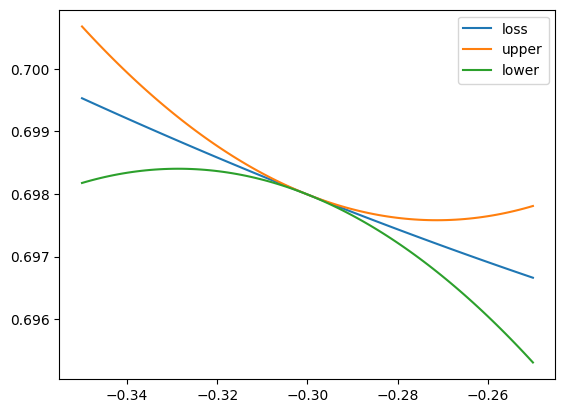
We plot the upper and lower bounds in the Quadratic Bound for Smooth Functions around \(x = x_0\). It turns out we can take \(L=1\) because all features are uniformly random between \(-1\) and \(1\). Observe that minimizing the upper quadratic bound leads to a decrease in \(\mathcal{L}\).
x0 = -0.3
x = np.linspace(x0-0.05,x0+0.05,100)
upper = loss(x0,a,b) + (x - x0)*grad(x0,a,b) + (1/2)*(x - x0)**2
lower = loss(x0,a,b) + (x - x0)*grad(x0,a,b) - (1/2)*(x - x0)**2

plt.plot(x, loss(x,a,b), label='loss')
plt.plot(x, upper, label='upper')
plt.plot(x, lower, label='lower')
plt.legend()
plt.show()

3.8.2.2. Logistic regression: another dataset#
Recall that to run gradient descent, we first implement a function computing a descent update. It takes as input a function grad_fn computing the gradient itself, as well as a current iterate and a step size. We now also feed a dataset as additional input.
def sigmoid(z):
    return 1/(1+np.exp(-z))

def desc_update_for_logreg(grad_fn, A, b, curr_x, beta):
    gradient = grad_fn(curr_x, A, b)
    return curr_x - beta*gradient

def gd_for_logreg(loss_fn, grad_fn, A, b, init_x, beta=1e-3, niters=int(1e5)):
    curr_x = init_x

    for iter in range(niters):
        curr_x = desc_update_for_logreg(grad_fn, A, b, curr_x, beta)

    return curr_x

def pred_fn(x, A):
    return sigmoid(A @ x)

def loss_fn(x, A, b):
    return np.mean(-b*np.log(pred_fn(x, A)) - (1 - b)*np.log(1 - pred_fn(x, A)))

def grad_fn(x, A, b):
    return -A.T @ (b - pred_fn(x, A))/len(b)

def stepsize_for_logreg(A, b):
    L = LA.norm(A)**2 / (4 * len(b))
    return 1/L
We analyze with a simple dataset from UC Berkeley’s DS100 course. The file lebron.csv is available here. Quoting a previous version of the course’s textbook:
In basketball, players score by shooting a ball through a hoop. One such player, LeBron James, is widely considered one of the best basketball players ever for his incredible ability to score. LeBron plays in the National Basketball Association (NBA), the United States’s premier basketball league. We’ve collected a dataset of all of LeBron’s attempts in the 2017 NBA Playoff Games using the NBA statistics website (https://stats.nba.com/).
We first load the data and look at its summary.
data = pd.read_csv('lebron.csv')
data.head()
| game_date | minute | opponent | action_type | shot_type | shot_distance | shot_made | |
|---|---|---|---|---|---|---|---|
| 0 | 20170415 | 10 | IND | Driving Layup Shot | 2PT Field Goal | 0 | 0 |
| 1 | 20170415 | 11 | IND | Driving Layup Shot | 2PT Field Goal | 0 | 1 |
| 2 | 20170415 | 14 | IND | Layup Shot | 2PT Field Goal | 0 | 1 |
| 3 | 20170415 | 15 | IND | Driving Layup Shot | 2PT Field Goal | 0 | 1 |
| 4 | 20170415 | 18 | IND | Alley Oop Dunk Shot | 2PT Field Goal | 0 | 1 |
data.describe()
| game_date | minute | shot_distance | shot_made | |
|---|---|---|---|---|
| count | 3.840000e+02 | 384.00000 | 384.000000 | 384.000000 |
| mean | 2.017052e+07 | 24.40625 | 10.695312 | 0.565104 |
| std | 6.948501e+01 | 13.67304 | 10.547586 | 0.496390 |
| min | 2.017042e+07 | 1.00000 | 0.000000 | 0.000000 |
| 25% | 2.017050e+07 | 13.00000 | 1.000000 | 0.000000 |
| 50% | 2.017052e+07 | 25.00000 | 6.500000 | 1.000000 |
| 75% | 2.017060e+07 | 35.00000 | 23.000000 | 1.000000 |
| max | 2.017061e+07 | 48.00000 | 31.000000 | 1.000000 |
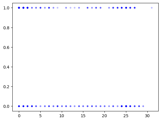
The two columns we will be interested in are shot_distance (LeBron’s distance from the basket when the shot was attempted (ft)) and shot_made (0 if the shot missed, 1 if the shot went in). As the summary table above indicates, the average distance was 10.6953 and the frequency of shots made was 0.565104. We extract those two columns and display them on a scatter plot.
feature = data['shot_distance']
label = data['shot_made']

plt.scatter(feature, label, s=10, color='b', alpha=0.2)
plt.show()

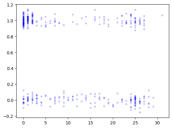
As you can see, this kind of data is hard to vizualize because of the superposition of points with the same \(x\) and \(y\)-values. One trick is to jiggle the \(y\)’s a little bit by adding Gaussian noise. We do this next and plot again.
seed = 535
rng = np.random.default_rng(seed)

label_jitter = label + 0.05*rng.normal(0,1,len(label))

plt.scatter(feature, label_jitter, s=10, color='b', alpha=0.2)
plt.show()

We apply GD to logistic regression. We first construct the data matrices \(A\) and \(\mathbf{b}\). To allow an affine function of the features, we add a column of \(1\)’s as we have done before.
A = np.stack((np.ones(len(label)),feature),axis=-1)
b = label
We run GD starting from \((0,0)\) with a step size computed from the smoothness of the objective as above.
stepsize = stepsize_for_logreg(A, b)
print(stepsize)
0.017671625306319678
init_x = np.zeros(A.shape[1])
best_x = gd_for_logreg(loss_fn, grad_fn, A, b, init_x, beta=stepsize)
print(best_x)
[ 0.90959003 -0.05890828]
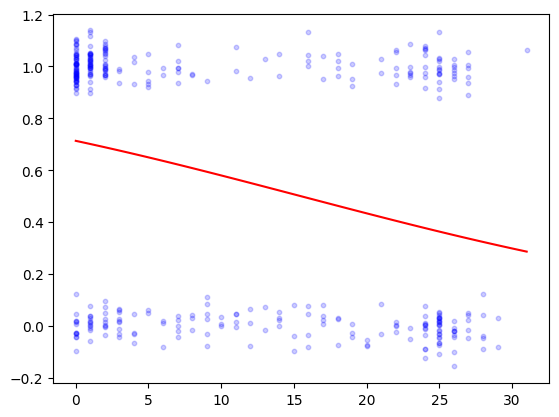
Finally we plot the results.
grid = np.linspace(np.min(feature), np.max(feature), 100)
feature_grid = np.stack((np.ones(len(grid)),grid),axis=-1)
predict_grid = sigmoid(feature_grid @ best_x)

plt.scatter(feature, label_jitter, s=10, color='b', alpha=0.2)
plt.plot(grid,predict_grid,'r')
plt.show()

