Online suppplementary material

2.7. Online suppplementary material#

2.7.1. Quizzes, solutions, code, etc.#

2.7.1.1. Just the code#

An interactive Jupyter notebook featuring the code in this chapter can be accessed below (Google Colab recommended). You are encouraged to tinker with it. Some suggested computational exercises are scattered throughout. The notebook is also available as a slideshow.

2.7.1.2. Self-assessment quizzes#

A more extensive web version of the self-assessment quizzes is available by following the links below.

2.7.1.3. Auto-quizzes#

Automatically generated quizzes for this chapter can be accessed here (Google Colab recommended).

Auto-quizzes (Open In Colab)

2.7.1.4. Solutions to odd-numbered warm-up exercises#

(with help from Claude, Gemini, and ChatGPT)

Answer and justification for E2.2.1: Yes, $U$ is a linear subspace of $\mathbb{R}^3$. Let $u_1 = (x_1, y_1, z_1), u_2 = (x_2, y_2, z_2) \in U$ and $\alpha \in \mathbb{R}$. Then

\[\begin{align*} x_1 + 2y_1 - z_1 &= 0 \\ x_2 + 2y_2 - z_2 &= 0 \\ \alpha(x_1 + 2y_1 - z_1) + (x_2 + 2y_2 - z_2) &= 0 \\ (\alpha x_1 + x_2) + 2(\alpha y_1 + y_2) - (\alpha z_1 + z_2) &= 0 \end{align*}\]

So $\alpha u_1 + u_2 \in U$, proving $U$ is a linear subspace.

Answer and justification for E2.2.3: One basis for $U$ is $\{(1, 1, 0), (1, 0, 1)\}$. Any vector $(x, y, z) \in U$ can be written as

\[\begin{align*} (x, y, z) &= (y-z, y, z) \\ &= y(1, 1, 0) + z(1, 0, 1) \end{align*}\]

So $\{(1, 1, 0), (1, 0, 1)\}$ spans $U$. They are also linearly independent, as $\alpha(1, 1, 0) + \beta(1, 0, 1) = 0$ implies $\alpha = \beta = 0$. Thus, this is a basis for $U$.

Answer and justification for E2.2.5: Yes, $u_1$ and $u_2$ form an orthonormal list. We have

\[\begin{align*} \|u_1\| &= \sqrt{(1/\sqrt{2})^2 + (1/\sqrt{2})^2} = 1 \\ \|u_2\| &= \sqrt{(1/\sqrt{2})^2 + (-1/\sqrt{2})^2} = 1 \\ \langle u_1, u_2 \rangle &= (1/\sqrt{2})(1/\sqrt{2}) + (1/\sqrt{2})(-1/\sqrt{2}) = 0 \end{align*}\]

So $u_1$ and $u_2$ are unit vectors and are orthogonal to each other.

Answer and justification for E2.2.7: $A$ is nonsingular. Its columns are $(1, 3)$ and $(2, 4)$, which are linearly independent

\[\begin{align*} \alpha(1, 3) + \beta(2, 4) &= (0, 0) \\ \alpha + 2\beta &= 0 \\ 3\alpha + 4\beta &= 0 \end{align*}\]

This system has only the trivial solution $\alpha = \beta = 0$. So the columns of $A$ are linearly independent, and since $A$ is a $2 \times 2$ matrix, this means it has rank 2 and is nonsingular.

Answer and justification for E2.2.9:

\[ \mathbf{v} = \alpha \mathbf{w}_1 + \beta \mathbf{w}_2 \implies (2, 3, 5) = \alpha (1, 0, 1) + \beta (0, 1, 1). \]

Solving the system of equations

\[ 2 = \alpha, \quad 3 = \beta, \quad 5 = \alpha + \beta. \]

Substitute $\alpha = 2$ and $\beta = 3$ into the third equation

\[ 5 = 2 + 3 \implies \alpha = 2, \beta = 3. \]

Thus, $\mathbf{v} = 2\mathbf{w}_1 + 3\mathbf{w}_2$.

Answer and justification for E2.2.11:

Solve $B \mathbf{x} = \mathbf{0}$

\[\begin{split} \begin{pmatrix} 1 & 2 & 3 \\ 4 & 5 & 6 \end{pmatrix} \begin{pmatrix} x_1 \\ x_2 \\ x_3 \end{pmatrix} = \begin{pmatrix} 0 \\ 0 \end{pmatrix}. \end{split}\]

This gives the system

\[ x_1 + 2x_2 + 3x_3 = 0, \]

\[ 4x_1 + 5x_2 + 6x_3 = 0. \]

Solving, we get $x_1 = -x_3$, $x_2 = 0$, and $x_3 = x_3$. The null space is spanned by $\begin{pmatrix} -1 \\ 0 \\ 1 \end{pmatrix}$.

Answer and justification for E2.2.13: Consider the equation $\alpha_1\mathbf{u}_1 + \alpha_2\mathbf{u}_2 + \alpha_3\mathbf{u}_3 = 0$. This leads to the system of equations

\[ \alpha_1 + 2\alpha_2 + \alpha_3 = 0 2\alpha_1 - \alpha_2 + 8\alpha_3 = 0 3\alpha_1 + 6\alpha_3 = 0 \]

Solving this system, we find that $\alpha_1 = -2\alpha_3$ and $\alpha_2 = \alpha_3$. Choosing $\alpha_3 = 1$, we get a non-trivial solution $\alpha_1 = -2$, $\alpha_2 = 1$, $\alpha_3 = 1$. Therefore, the vectors are linearly dependent.

Answer and justification for E2.2.15: We can write this system as $A\mathbf{x} = \mathbf{b}$, where $A = \begin{bmatrix} 2 & 1 \\ 1 & -1 \end{bmatrix}$, $\mathbf{x} = \begin{bmatrix} x \\ y \end{bmatrix}$, and $\mathbf{b} = \begin{bmatrix} 3 \\ 1 \end{bmatrix}$. Since $\det(A) = -3 \neq 0$, $A$ is invertible. We find that $A^{-1} = \frac{1}{-3} \begin{bmatrix} -1 & -1 \\ -1 & 2 \end{bmatrix}$.

Then, the solution is

\[\begin{split} \mathbf{x} = A^{-1}\mathbf{b} = \frac{1}{-3} \begin{bmatrix} -1 & -1 \\ -1 & 2 \end{bmatrix} \begin{bmatrix} 3 \\ 1 \end{bmatrix} = \begin{bmatrix} \frac{4}{3} \\ -\frac{1}{3} \end{bmatrix}. \end{split}\]

Answer and justification for E2.3.1: While

\[\begin{split} Q^T Q = \begin{pmatrix} 1 & 0\\ 0 & 1 \end{pmatrix} = I_{2 \times 2}, \end{split}\]

the matrix $Q$ is not square. Therefore, $Q$ is not an orthogonal matrix.

Answer and justification for E2.3.3:

\[ \mathrm{proj}_{U} \mathbf{v} = \frac{\langle \mathbf{v}, \mathbf{u} \rangle}{\|\mathbf{u}\|^2} \mathbf{u} = \frac{(2 \cdot 1 + 3 \cdot 1)}{(1^2 + 1^2)} \mathbf{u} = \frac{5}{2} (1, 1) = \left(\frac{5}{2}, \frac{5}{2}\right). \]

Answer and justification for E2.3.5: The projection of $\mathbf{v}$ onto $\mathbf{u}$ is given by

\[\begin{split} \text{proj}_{\mathbf{u}} \mathbf{v} = \frac{\langle \mathbf{u}, \mathbf{v} \rangle}{\|\mathbf{u}\|^2} \mathbf{u} = \frac{(1)(1) + (1)(2) + (0)(1)}{1^2 + 1^2 + 0^2} \begin{bmatrix} 1 \\ 1 \\ 0 \end{bmatrix} = \frac{3}{2} \begin{bmatrix} 1 \\ 1 \\ 0 \end{bmatrix} = \begin{bmatrix} \frac{3}{2} \\ \frac{3}{2} \\ 0 \end{bmatrix}. \end{split}\]

Answer and justification for E2.3.7: Using the orthonormal basis $\{q_1, q_2\}$ for $U$ from the text, we have: $$\mathrm{proj}_U v = \langle v, q_1 \rangle q_1 + \langle v, q_2 \rangle q_2 = \frac{4}{\sqrt{2}} \cdot \frac{1}{\sqrt{2}}(1, 0, 1) + \frac{5}{\sqrt{6}} \cdot \frac{1}{\sqrt{6}}(-1, 2, 1) = (\frac{7}{3}, \frac{10}{3}, \frac{13}{3}).$$

Answer and justification for E2.3.9: From E2.3.7 and E2.3.8, we have:

\[ \mathrm{proj}_U v = (\frac{7}{3}, \frac{10}{3}, \frac{13}{3})^T, \quad v - \mathrm{proj}_U v = (-\frac{1}{3}, -\frac{1}{3}, \frac{2}{3})^T. \]

Computing the squared norms:

\[ \|v\|^2 = 1^2 + 2^2 + 3^2 = 14, \quad \|\mathrm{proj}_U v\|^2 = (\frac{7}{3})^2 + (\frac{10}{3})^2 + (\frac{13}{3})^2 = \frac{146}{3}, \quad \|v - \mathrm{proj}_U v\|^2 = (-\frac{1}{3})^2 + (-\frac{1}{3})^2 + (\frac{2}{3})^2 = \frac{2}{3}. \]

Indeed, $\|v\|^2 = 14 = \frac{146}{3} + \frac{2}{3} = \|\mathrm{proj}_U v\|^2 + \|v - \mathrm{proj}_U v\|^2$, verifying the Pythagorean theorem.

Answer and justification for E2.3.11: Since $\mathbf{u}_1$ is not a unit vector, we first normalize it: $\mathbf{q}_1 = \frac{\mathbf{u}_1}{\|\mathbf{u}_1\|} = \frac{1}{3}\begin{pmatrix} 2 \\ 1 \\ -2 \end{pmatrix}$. Then, $\mathrm{proj}_{\mathbf{u}_1} \mathbf{u}_2 = \langle \mathbf{u}_2, \mathbf{q}_1 \rangle \mathbf{q}_1 = \frac{1}{9} \begin{pmatrix} 2 \\ 1 \\ -2 \end{pmatrix}$.

Answer and justification for E2.3.13: We want to find all vectors $\begin{pmatrix} x \\ y \\ z \end{pmatrix}$ such that $\begin{pmatrix} x \\ y \\ z \end{pmatrix} \cdot \begin{pmatrix} 1 \\ 1 \\ 0 \end{pmatrix} = 0$. This gives us the equation $x + y = 0$, or $x = -y$. Thus, any vector of the form $\begin{pmatrix} -y \\ y \\ z \end{pmatrix} = y\begin{pmatrix} -1 \\ 1 \\ 0 \end{pmatrix} + z\begin{pmatrix} 0 \\ 0 \\ 1 \end{pmatrix}$ is in $W^\perp$. So, a basis for $W^\perp$ is $\left\{\begin{pmatrix} -1 \\ 1 \\ 0 \end{pmatrix}, \begin{pmatrix} 0 \\ 0 \\ 1 \end{pmatrix}\right\}$.

Answer and justification for E2.3.15:

\[\begin{split} A^T A = \begin{pmatrix} 1 & 1 \\ 1 & -1 \end{pmatrix}^T \begin{pmatrix} 1 & 1 \\ 1 & -1 \end{pmatrix} = \begin{pmatrix} 2 & 0 \\ 0 & 2 \end{pmatrix}, \quad A^T \mathbf{b} = \begin{pmatrix} 1 & 1 \\ 1 & -1 \end{pmatrix}^T \begin{pmatrix} 3 \\ 1 \end{pmatrix} = \begin{pmatrix} 4 \\ 2 \end{pmatrix}. \end{split}\]

Thus, $\mathbf{x} = (A^T A)^{-1} A^T \mathbf{b} = \begin{pmatrix} 2 & 0 \\ 0 & 2 \end{pmatrix}^{-1} \begin{pmatrix} 4 \\ 2 \end{pmatrix} = \begin{pmatrix} 2 \\ 1 \end{pmatrix}$.

Answer and justification for E2.4.1: $\mathbf{q}_1 = \frac{\mathbf{a}_1}{\|\mathbf{a}_1\|} = (1, 0)$, $\mathbf{v}_2 = \mathbf{a}_2 - \langle \mathbf{q}_1, \mathbf{a}_2 \rangle \mathbf{q}_1 = (0, 1)$, $\mathbf{q}_2 = \frac{\mathbf{v}_2}{\|\mathbf{v}_2\|} = (0, 1)$.

Answer and justification for E2.4.3: Let $w_1 = (1, 1)$ and $w_2 = (1, 0)$. Then

\[\begin{align*} q_1 &= \frac{w_1}{\|w_1\|} = (\frac{1}{\sqrt{2}}, \frac{1}{\sqrt{2}}) \\ q_2 &= \frac{w_2 - \langle w_2, q_1 \rangle q_1}{\|w_2 - \langle w_2, q_1 \rangle q_1\|} \\ &= \frac{(1, 0) - (\frac{1}{\sqrt{2}})(\frac{1}{\sqrt{2}}, \frac{1}{\sqrt{2}})}{\sqrt{1 - (\frac{1}{\sqrt{2}})^2}} \\ &= (\frac{1}{\sqrt{2}}, -\frac{1}{\sqrt{2}}) \end{align*}\]

So $\{q_1, q_2\}$ is an orthonormal basis.

Answer and justification for E2.4.5: Using the orthonormal basis $\{q_1, q_2\}$ from E2.4.4, we have $Q = [q_1\ q_2]$. To find $R$, we observe that $a_1 = \sqrt{3}q_1$ and $a_2 = \frac{1}{\sqrt{3}}q_1 + \frac{5}{\sqrt{21}}q_2$. Therefore, $R = \begin{pmatrix} \sqrt{3} & \frac{1}{\sqrt{3}} \\ 0 & \frac{5}{\sqrt{21}} \end{pmatrix}$.

Answer and justification for E2.4.7: $\mathbf{x} = (2, 1)$. From the second equation, $3x_2 = 3$, so $x_2 = 1$. Substituting into the first equation, $2x_1 - 1 = 4$, so $x_1 = 2$.

Answer and justification for E2.4.9: $H = I_{3 \times 3} - 2\mathbf{z}\mathbf{z}^T/\|\mathbf{z}\|^2 = \begin{pmatrix} 0 & 1 & 0 \\ 1 & 0 & 0 \\ 0 & 0 & 1 \end{pmatrix}$.

Answer and justification for E2.4.11: To verify that $H_1$ is orthogonal, we check if $H_1^T H_1 = I_{2 \times 2}$:

\[\begin{split} H_1^T H_1 = \begin{pmatrix} \frac{7}{5} & -\frac{6}{5} \\ -\frac{6}{5} & -\frac{1}{5} \end{pmatrix} \begin{pmatrix} \frac{7}{5} & -\frac{6}{5} \\ -\frac{6}{5} & -\frac{1}{5} \end{pmatrix} = \begin{pmatrix} 1 & 0 \\ 0 & 1 \end{pmatrix} = I_{2 \times 2}. \end{split}\]

To verify that $H_1$ is symmetric, we check if $H_1^T = H_1$, which is true by observation.

Answer and justification for E2.4.13: We have $H_1 A = R$, where $R = \begin{pmatrix} -\frac{\sqrt{10}}{5} & -\frac{2}{\sqrt{10}} \\ 0 & \frac{14}{5} \end{pmatrix}$ is upper triangular. Therefore, $Q^T = H_1$, and $Q = H_1^T = \begin{pmatrix} \frac{7}{5} & \frac{6}{5} \\ -\frac{6}{5} & \frac{1}{5} \end{pmatrix}$.

Answer and justification for E2.4.15: Let $\mathbf{y}_1 = (3, 4)^T$ be the first column of $A$. Then $\mathbf{z}_1 = \|\mathbf{y}_1\| \mathbf{e}_1^{(2)} - \mathbf{y}_1 = (5, -4)^T$ and $H_1 = I_{2 \times 2} - 2\mathbf{z}_1\mathbf{z}_1^T / \|\mathbf{z}_1\|^2 = \begin{pmatrix} 3/5 & 4/5 \\ 4/5 & -3/5 \end{pmatrix}$. We can verify that $H_1 A = \begin{pmatrix} 5 & 1 \\ 0 & -2/5 \end{pmatrix}$.

Answer and justification for E2.4.17:

\[\begin{align*} Q &= \begin{pmatrix} \frac{1}{\sqrt{2}} & \frac{1}{\sqrt{2}} \\ \frac{1}{\sqrt{2}} & -\frac{1}{\sqrt{2}} \end{pmatrix}, \\ R &= Q^T A = \begin{pmatrix} \sqrt{2} & 0 \\ 0 & \sqrt{2} \end{pmatrix}, \\ Q^T \mathbf{b} &= \begin{pmatrix} \frac{1}{\sqrt{2}} & \frac{1}{\sqrt{2}} \\ \frac{1}{\sqrt{2}} & -\frac{1}{\sqrt{2}} \end{pmatrix} \begin{pmatrix} 2 \\ 0 \end{pmatrix} = \begin{pmatrix} \sqrt{2} \\ \sqrt{2} \end{pmatrix}, \\ R x &= Q^T \mathbf{b}, \quad \begin{pmatrix} \sqrt{2} & 0 \\ 0 & \sqrt{2} \end{pmatrix} x = \begin{pmatrix} \sqrt{2} \\ \sqrt{2} \end{pmatrix}, \\ x &= \begin{pmatrix} 1 \\ 1 \end{pmatrix}. \end{align*}\]

The solution is $x = \begin{pmatrix} 1 \\ 1 \end{pmatrix}$.

Answer and justification for E2.5.1:

\[\begin{split} A = \begin{pmatrix} 1 & 1 \\ 1 & 2 \\ 1 & 3 \\ 1 & 4 \end{pmatrix}, \quad y = \begin{pmatrix} 2 \\ 4 \\ 5 \\ 7 \end{pmatrix}. \end{split}\]

The normal equations are:

\[\begin{split} A^T A \beta = A^T y \Rightarrow \begin{pmatrix} 4 & 10 \\ 10 & 30 \end{pmatrix} \begin{pmatrix} \beta_0 \\ \beta_1 \end{pmatrix} = \begin{pmatrix} 18 \\ 47 \end{pmatrix}. \end{split}\]

Solving this system of equations yields $\beta_0 = \frac{1}{2}$ and $\beta_1 = \frac{3}{2}$.

Answer and justification for E2.5.3:

\[\begin{split} A = \begin{bmatrix} 1 & 1 \\ 1 & 2 \\ 1 & 3 \end{bmatrix}, \quad \boldsymbol{\beta} = \begin{bmatrix} \beta_0 \\ \beta_1 \end{bmatrix}, \quad \mathbf{y} = \begin{bmatrix} 3 \\ 5 \\ 8 \end{bmatrix} \end{split}\]

This follows from the linear regression model $y_i = \beta_0 + \beta_1 x_i + \epsilon_i$ for each data point.

Answer and justification for E2.5.5:

\[\begin{split} \boldsymbol{\beta} = \begin{bmatrix} \beta_0 \\ \beta_1 \end{bmatrix} = (A^T A)^{-1} A^T \mathbf{y} = \begin{bmatrix} 1 \\ 2 \end{bmatrix} \end{split}\]

We solve the linear system by inverting $A^T A$ and multiplying by $A^T \mathbf{y}$.

Answer and justification for E2.5.7:

\[\begin{split} A = \begin{bmatrix} 1 & -1 & 1 \\ 1 & 0 & 0 \\ 1 & 1 & 1 \end{bmatrix} \end{split}\]

For a quadratic model, we need columns for $1$, $x$, and $x^2$.

Answer and justification for E2.5.9: We solve the normal equations $A^T A \beta = A^T \mathbf{y}$.

\[\begin{align*} A^T A &= \begin{pmatrix} 1 & 1 & 1 \\ 1 & 2 & 3 \end{pmatrix} \begin{pmatrix} 1 & 1 \\ 1 & 2 \\ 1 & 3 \end{pmatrix} = \begin{pmatrix} 3 & 6 \\ 6 & 14 \end{pmatrix}, \\ A^T \mathbf{y} &= \begin{pmatrix} 1 & 1 & 1 \\ 1 & 2 & 3 \end{pmatrix} \begin{pmatrix} 1 \\ 2 \\ 3 \end{pmatrix} = \begin{pmatrix} 6 \\ 14 \end{pmatrix}. \end{align*}\]

Solving $\begin{pmatrix} 3 & 6 \\ 6 & 14 \end{pmatrix} \beta = \begin{pmatrix} 6 \\ 14 \end{pmatrix}$:

\[\begin{align*} \beta &= \begin{pmatrix} \beta_0 \\ \beta_1 \end{pmatrix} = \begin{pmatrix} 0 \\ 1 \end{pmatrix}. \end{align*}\]

Answer and justification for E2.5.11: Compute the predicted $y$ values:

\[\begin{align*} \hat{y}_1 &= 2(1) + 1 = 3, \\ \hat{y}_2 &= 2(2) + 1 = 5, \\ \hat{y}_3 &= 2(3) + 1 = 7. \end{align*}\]

Compute the residuals:

\[\begin{align*} r_1 &= 3 - 3 = 0, \\ r_2 &= 5 - 5 = 0, \\ r_3 &= 7 - 7 = 0. \end{align*}\]

RSS is:

\[\begin{align*} \mathrm{RSS} &= 0^2 + 0^2 + 0^2 = 0. \end{align*}\]

2.7.1.5. Learning outcomes#

Define the concepts of linear subspaces, spans, and bases in vector spaces.
Check the conditions for a set of vectors to be linearly independent or form a basis of a vector space.
Define the inverse of a nonsingular matrix and prove its uniqueness.
Define the dimension of a linear subspace.
State the Pythagorean Theorem.
Verify whether a given list of vectors is orthonormal.
Derive the coefficients in an orthonormal basis expansion of a vector.
Apply the Gram-Schmidt process to transform a basis into an orthonormal basis.
Prove key theorems related to vector spaces and matrix inverses, such as the Pythagorean theorem for orthogonal vectors and the conditions for linear independence in matrix columns.
Illustrate examples of linear subspaces and their bases, using both theoretical definitions and numerical examples.
Define the orthogonal projection of a vector onto a linear subspace and characterize it geometrically.
Compute the orthogonal projection of a vector onto a linear subspace spanned by an orthonormal list of vectors.
Illustrate the process of finding the orthogonal projection of a vector onto a subspace using geometric intuition.
Prove the uniqueness of the orthogonal projection.
Express the orthogonal projection in matrix form.
Define the orthogonal complement of a linear subspace and find an orthonormal basis for it.
State and prove the Orthogonal Decomposition Lemma, and use it to decompose a vector into its orthogonal projection and a vector in the orthogonal complement.
Formulate the linear least squares problem as an optimization problem and derive the normal equations.
Apply the concepts of orthogonal projection and orthogonal complement to solve overdetermined systems using the least squares method.
Determine the uniqueness of the least squares solution based on the linear independence of the columns of the matrix.
Implement the Gram-Schmidt algorithm to obtain an orthonormal basis from a set of linearly independent vectors.
Express the Gram-Schmidt algorithm using a matrix factorization perspective, known as the QR decomposition.
Apply the QR decomposition to solve linear least squares problems as an alternative to the normal equations approach.
Define Householder reflections and explain their role in introducing zeros below the diagonal of a matrix.
Construct a QR decomposition using a sequence of Householder transformations.
Compare the numerical stability of the Gram-Schmidt algorithm and the Householder transformations approach for computing the QR decomposition.
Formulate the linear regression problem as a linear least squares optimization problem.
Extend the linear regression model to polynomial regression by incorporating higher-degree terms and interaction terms in the design matrix.
Recognize and explain the issue of overfitting in polynomial regression and its potential consequences.
Apply the least squares method to simulated data and real-world datasets, such as the Advertising dataset, to estimate regression coefficients.
Understand and implement the bootstrap method for linear regression to assess the variability of estimated coefficients and determine the statistical significance of the results.

$\aleph$

2.7.2. Additional sections#

2.7.2.1. Orthogonality in high dimension#

In high dimension, orthogonality – or more accurately near-orthogonality – is more common than one might expect. We illustrate this phenomenon here.

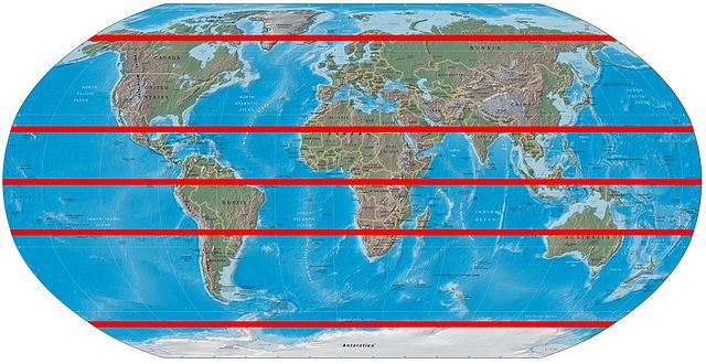
Let $\mathbf{X}$ be a standard Normal $d$-vector. Its joint PDF depends only on the its norm $\|\mathbf{X}\|$. So $\mathbf{Y} = \frac{\mathbf{X}}{\|\mathbf{X}\|}$ is uniformly distributed over the $(d-1)$-sphere $\mathcal{S} = \{\mathbf{x}\in \mathbb{R}^d:\|\mathbf{x}\|=1\}$, that is, the surface of the unit $d$-ball centered aroungd the origin. We write $\mathbf{Y} \sim \mathrm{U}[\mathcal{S}]$. The following theorem shows that if we take two independent samples $\mathbf{Y}_1, \mathbf{Y}_2 \sim \mathrm{U}[\mathcal{S}]$ they are likely to be nearly orthogonal when $d$ is large, that is, $|\langle\mathbf{Y}_1, \mathbf{Y}_2\rangle|$ is likely to be small. By symmetry, there is no loss of generality in taking one of the two vectors to be the north pole $\mathbf{e}_d = (0,\ldots,0,1)$. A different way to state the theorem is that most of the mass of the $(d-1)$-sphere is in a small band around the equator.

Figure: Band around the equator (Source)

$\bowtie$

THEOREM (Orthogonality in High Dimension) Let $\mathcal{S} = \{\mathbf{x}\in \mathbb{R}^d:\|\mathbf{x}\|=1\}$ and $\mathbf{Y} \sim \mathrm{U}[\mathcal{S}]$. Then for any $\varepsilon > 0$, as $d \to +\infty$,

\[ \mathbb{P}[|\langle\mathbf{Y}, \mathbf{e}_d\rangle| \geq \varepsilon] \to 0. \]

$\sharp$

Proof idea: We write $\mathbf{Y}$ in terms of a standard Normal. Its squared norm is a sum of independent random variables. After bringing it to the numerator, we can apply Chebyshev.

Proof: Recall that $\mathbf{Y}$ is $\frac{\mathbf{X}}{\|\mathbf{X}\|}$ where $\mathbf{X}$ is a standard Normal $d$-vector. The probability we want to bound can be re-written as

\[\begin{align*} \mathbb{P}[|\langle\mathbf{Y}, \mathbf{e}_d\rangle| \geq \varepsilon] &= \mathbb{P}\left[\left|\left\langle\frac{\mathbf{X}}{\|\mathbf{X}\|}, \mathbf{e}_d\right\rangle\right|^2 \geq \varepsilon^2\right]\\ &= \mathbb{P}\left[\left|\frac{\langle\mathbf{X},\mathbf{e}_d\rangle}{\|\mathbf{X}\|}\right|^2 \geq \varepsilon^2\right]\\ &= \mathbb{P}\left[\frac{X_d^2}{\sum_{j=1}^d X_j^2} \geq \varepsilon^2\right]\\ &= \mathbb{P}\left[X_d^2 \geq \varepsilon^2 \sum_{j=1}^d X_j^2\right]\\ &= \mathbb{P}\left[\sum_{j=1}^{d-1} (-\varepsilon^2 X_j^2) + (1-\varepsilon^2) X_d^2 \geq 0\right]. \end{align*}\]

We are now looking at a sum of independent (but not identically distributed) random variables

\[ Z = \sum_{j=1}^{d-1} (-\varepsilon^2 X_j^2) + (1-\varepsilon^2) X_d^2 \]

and we can appeal to our usual Chebyshev machinery. The expectation is, by linearity,

\[ \mathbb{E}[Z] = - \sum_{j=1}^{d-1} \varepsilon^2 \mathbb{E}[X_j^2] + (1-\varepsilon^2) \mathbb{E}[X_d^2] = \{- (d-1) \,\varepsilon^2 + (1-\varepsilon^2)\} \]

where we used that $X_1,\ldots,X_d$ are standard Normal variables and that, in particular, their mean is $0$ and their variance is $1$ so that $\mathbb{E}[X_1^2] = 1$.

The variance is, by independence of the $X_j$’s,

\[\begin{align*} \mathrm{Var}[Z] &= \sum_{j=1}^{d-1} \varepsilon^4 \mathrm{Var}[X_j^2] + (1-\varepsilon^2)^2 \mathrm{Var}[X_d^2]\\ &= \{(d-1) \,\varepsilon^4 + (1-\varepsilon^2)^2\}\mathrm{Var}[X_1^2]. \end{align*}\]

So by Chebyshev

\[\begin{align*} \mathbb{P}\left[Z \geq 0\right] &\leq \mathbb{P}\left[\left|Z - \mathbb{E}[Z]\right|\geq |\mathbb{E}[Z]|\right]\\ &\leq \frac{\mathrm{Var}[Z]}{\mathbb{E}[Z]^2}\\ &= \frac{\{(d-1) \,\varepsilon^4 + (1-\varepsilon^2)^2\} \mathrm{Var}[X_1^2]}{\{- (d-1) \,\varepsilon^2 + (1-\varepsilon^2)\}^2}\\ &\to 0 \end{align*}\]

as $d \to +\infty$. To get the limit we observed that, for large $d$, the deminator scales like $d^2$ while the numerator scales only like $d$. $\square$

2.7.2.2. Bootstrapping for linear regression#

We return to the linear case, but with the full set of predictors.

data = pd.read_csv('advertising.csv')
TV = data['TV'].to_numpy()
sales = data['sales'].to_numpy()
n = np.size(TV)

radio = data['radio'].to_numpy()
newspaper = data['newspaper'].to_numpy()

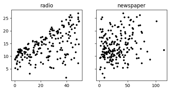
f, (ax1, ax2) = plt.subplots(1, 2, sharex=False, sharey=True, figsize=(6.5,3))
ax1.scatter(radio, sales, s=10, c='k')
ax2.scatter(newspaper, sales, s=10, c='k')
ax1.set_title('radio'), ax2.set_title('newspaper')
plt.show()

../../_images/155aab1286ee6a73580fa8d8e6151412c1f8ba7fe6e98a24fa26dd25ee5d2fd4.png

A = np.stack((np.ones(n), TV, radio, newspaper), axis=-1)
coeff = mmids.ls_by_qr(A,sales)
print(coeff)

[ 2.93888937e+00  4.57646455e-02  1.88530017e-01 -1.03749304e-03]

Newspaper advertising (the last coefficient) seems to have a much weaker effect on sales per dollar spent. Next, we briefly sketch one way to assess the statistical significance of such a conclusion.

Our coefficients are estimated from a sample. There is intrinsic variability in our sampling procedure. We would like to understand how our estimated coefficients compare to the true coefficients. This is set up beautifully in [Data8, Section 13.2]:

A data scientist is using the data in a random sample to estimate an unknown parameter. She uses the sample to calculate the value of a statistic that she will use as her estimate. Once she has calculated the observed value of her statistic, she could just present it as her estimate and go on her merry way. But she’s a data scientist. She knows that her random sample is just one of numerous possible random samples, and thus her estimate is just one of numerous plausible estimates. By how much could those estimates vary? To answer this, it appears as though she needs to draw another sample from the population, and compute a new estimate based on the new sample. But she doesn’t have the resources to go back to the population and draw another sample. It looks as though the data scientist is stuck. Fortunately, a brilliant idea called the bootstrap can help her out. Since it is not feasible to generate new samples from the population, the bootstrap generates new random samples by a method called resampling: the new samples are drawn at random from the original sample.

Without going into full details (see [DS100, Section 17.3] for more), it works as follows. Let $\{(\mathbf{x}_i, y_i)\}_{i=1}^n$ be our data. We assume that our sample is representative of the population and we simulate our sampling procedure by resampling from the sample. That is, we take a random sample with replacement $\mathcal{X}_{\mathrm{boot},1} = \{(\mathbf{x}_i, y_i)\,:\,i \in I\}$ where $I$ is a multi-set of elements from $[n]$ of size $n$. We recompute our estimated coefficients on $\mathcal{X}_{\mathrm{boot},1}$. Then we repeat independently for a desired number of replicates $\mathcal{X}_{\mathrm{boot},1}, \ldots, \mathcal{X}_{\mathrm{boot},r}$. Plotting a histogram of the resulting coefficients gives some idea of the variability of our estimates.

We implement the bootstrap for linear regression in Python next.

def linregboot(rng, A, b, replicates = np.int32(10000)):
    n,m = A.shape
    coeff_boot = np.zeros((m,replicates))
    for i in range(replicates):
        resample = rng.integers(0,n,n)
        Aboot = A[resample,:]
        bboot = b[resample]
        coeff_boot[:,i] = mmids.ls_by_qr(Aboot,bboot)
    return coeff_boot

First, let’s use a simple example with a known ground truth.

seed = 535
rng = np.random.default_rng(seed)

n, b0, b1 = 100, -1, 1
x = np.linspace(0,10,num=n)
y = b0 + b1*x + rng.normal(0,1,n)
A = np.stack((np.ones(n),x),axis=-1)

The estimated coefficients are the following.

coeff = mmids.ls_by_qr(A,y)
print(coeff)

[-1.03381171  1.01808039]

Now we apply the bootstrap and plot histograms of the two coefficients.

coeff_boot = linregboot(rng, A,y)

f, (ax1, ax2) = plt.subplots(1, 2, sharex=False, sharey=True, figsize=(7,3))
ax1.hist(coeff_boot[0,:], bins=20, color='lightblue', edgecolor='black')
ax2.hist(coeff_boot[1,:], bins=20, color='lightblue', edgecolor='black')
ax1.set_title('coeff1'), ax2.set_title('coeff2')
plt.show()

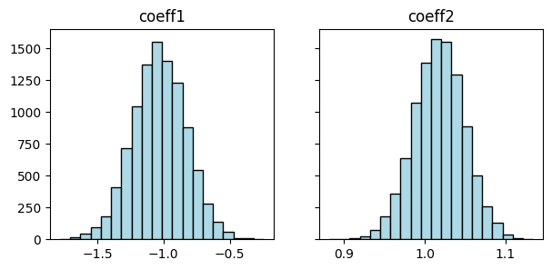
../../_images/6e70475b7474054cf0c761debe072019bfa7b678bf5713aad479715872c9389f.png

We see in the histograms that the true coefficient values $-1$ and $1$ fall within the likely range.

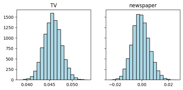
We return to the Advertising dataset and apply the bootstrap. Plotting a histogram of the coefficients corresponding to newspaper advertising shows that $0$ is a plausible value, while it is not for TV advertising.

n = np.size(TV)
A = np.stack((np.ones(n), TV, radio, newspaper), axis=-1)
coeff = mmids.ls_by_qr(A,sales)
print(coeff)

[ 2.93888937e+00  4.57646455e-02  1.88530017e-01 -1.03749304e-03]

coeff_boot = linregboot(rng, A,sales)

f, (ax1, ax2) = plt.subplots(1, 2, sharex=False, sharey=True, figsize=(7,3))
ax1.hist(coeff_boot[1,:], bins=20, color='lightblue', edgecolor='black')
ax2.hist(coeff_boot[3,:], bins=20, color='lightblue', edgecolor='black')
ax1.set_title('TV'), ax2.set_title('newspaper')
plt.show()

../../_images/9bbf02546f7e9282f6e04dca74639b03b9115c1b472aa52ccc94a555ac4422f5.png