
\(\newcommand{\bmu}{\boldsymbol{\mu}}\) \(\newcommand{\bSigma}{\boldsymbol{\Sigma}}\) \(\newcommand{\bfbeta}{\boldsymbol{\beta}}\) \(\newcommand{\bflambda}{\boldsymbol{\lambda}}\) \(\newcommand{\bgamma}{\boldsymbol{\gamma}}\) \(\newcommand{\bsigma}{{\boldsymbol{\sigma}}}\) \(\newcommand{\bpi}{\boldsymbol{\pi}}\) \(\newcommand{\btheta}{{\boldsymbol{\theta}}}\) \(\newcommand{\bphi}{\boldsymbol{\phi}}\) \(\newcommand{\balpha}{\boldsymbol{\alpha}}\) \(\newcommand{\blambda}{\boldsymbol{\lambda}}\) \(\renewcommand{\P}{\mathbb{P}}\) \(\newcommand{\E}{\mathbb{E}}\) \(\newcommand{\indep}{\perp\!\!\!\perp} \newcommand{\bx}{\mathbf{x}}\) \(\newcommand{\bp}{\mathbf{p}}\) \(\renewcommand{\bx}{\mathbf{x}}\) \(\newcommand{\bX}{\mathbf{X}}\) \(\newcommand{\by}{\mathbf{y}}\) \(\newcommand{\bY}{\mathbf{Y}}\) \(\newcommand{\bz}{\mathbf{z}}\) \(\newcommand{\bZ}{\mathbf{Z}}\) \(\newcommand{\bw}{\mathbf{w}}\) \(\newcommand{\bW}{\mathbf{W}}\) \(\newcommand{\bv}{\mathbf{v}}\) \(\newcommand{\bV}{\mathbf{V}}\) \(\newcommand{\bfg}{\mathbf{g}}\) \(\newcommand{\bfh}{\mathbf{h}}\) \(\newcommand{\horz}{\rule[.5ex]{2.5ex}{0.5pt}}\) \(\renewcommand{\S}{\mathcal{S}}\) \(\newcommand{\X}{\mathcal{X}}\) \(\newcommand{\var}{\mathrm{Var}}\) \(\newcommand{\pa}{\mathrm{pa}}\) \(\newcommand{\Z}{\mathcal{Z}}\) \(\newcommand{\bh}{\mathbf{h}}\) \(\newcommand{\bb}{\mathbf{b}}\) \(\newcommand{\bc}{\mathbf{c}}\) \(\newcommand{\cE}{\mathcal{E}}\) \(\newcommand{\cP}{\mathcal{P}}\) \(\newcommand{\bbeta}{\boldsymbol{\beta}}\) \(\newcommand{\bLambda}{\boldsymbol{\Lambda}}\) \(\newcommand{\cov}{\mathrm{Cov}}\) \(\newcommand{\bfk}{\mathbf{k}}\) \(\newcommand{\idx}[1]{}\) \(\newcommand{\xdi}{}\)
7.3. Limit behavior 1: stationary distributions#
We continue our exploration of basic Markov chain theory. In this section, we begin our study of the long-term behavior of a chain. As we did in the previous section, we restrict ourselves to finite-space discrete-time Markov chains that are also time-homogeneous.
7.3.1. Definitions#
An important property of Markov chains is that, when run for long enough, they converge to a sort of “equilibrium.” We develop parts of this theory here. What do we mean by “equilibrium”? Here is the key definition.
DEFINITION (Stationary Distribution) \(\idx{stationary distribution}\xdi\) Let \((X_t)_{t \geq 0}\) be a Markov chain on \(\mathcal{S} = [n]\) with transition matrix \(P = (p_{i,j})_{i,j=1}^n\). A probability distribution \(\bpi = (\pi_i)_{i=1}^n\) over \([n]\) is a stationary distribution of \((X_t)_{t \geq 0}\) (or of \(P\)) if:
\(\natural\)
In matrix form, this condition can be stated as
where recall that we think of \(\bpi\) as a row vector. One way to put this is that \(\bpi\) is a fixed point of \(P\) (through multiplication from the left). Another way to put it is that \(\bpi\) is a left (row) eigenvector of \(P\) with eigenvalue \(1\).
To see why a stationary distribution is indeed an equilibrium, we note the following.
LEMMA (Stationarity) \(\idx{stationarity lemma}\xdi\) Let \(\mathbf{z} \in \mathbb{R}^n\) be a left eigenvector of transition matrix \(P \in \mathbb{R}^{n \times n}\) with eigenvalue \(1\). Then \(\mathbf{z} P^s = \mathbf{z}\) for all integers \(s \geq 0\). \(\flat\)
Proof: Indeed,
\(\square\)
Suppose the initial distribution is equal to a stationary distribution \(\bpi\). Then, from the Time Marginals Theorem and the Stationarity Lemma, the distribution at any time \(s \geq 1\) is
That is, the distribution at all times indeed remains stationary.
In the next section we will derive a remarkable fact: under certain conditions, a Markov chain started from an arbitrary initial distribution converges in the limit of \(t \to +\infty\) to a stationary distribution.
EXAMPLE: (Weather Model, continued) Going back to the weather model, we compute a stationary distribution. We need \(\bpi = (\pi_1, \pi_2)^T\) to satisfy
that is,
You can check that, after rearranging, these two equations are in fact the same one.
Note, however, that we have some further restrictions: \(\bpi\) is a probability distribution. So \(\pi_1, \pi_2 \geq 0\) and \(\pi_1 + \pi_2 = 1\). Replacing the latter in the first equation we get
so that we require
And \(\pi_2 = 1 - \pi_1 = 1/2\). The second equation above is also automatically satisfied. \(\lhd\)
The previous example is quite special. It generalizes to all doubly stochastic matrices (including the Random Walk on the Petersen Graph for instance). Indeed, we claim that the uniform distribution is always a stationary distribution in the doubly stochastic case. Let \(P = (p_{i,j})_{i,j=1}^n\) be doubly stochastic over \([n]\) and let \(\bpi = (\pi_i)_{i=1}^n\) be the uniform distribution on \([n]\). Then for all \(j \in [n]\)
because the columns sum to \(1\). That proves the claim.
Is a stationary distribution guaranteed to exist? Is it unique? To answer this question, we first need some graph-theoretic concepts relevant to the long-term behavior of the chain.
DEFINITION (\(x \to y\)) A state \(x \in \S\) is said to communicate with a state \(y \in \S\) if there exists a sequence of states \(z_0 = x, z_1, z_2, \ldots, z_{r-1}, z_r = y\) such that for all \(\ell = 1,\ldots,r\)
We denote this property as \(x \to y\). \(\natural\)
In terms of the transition graph of the chain, the condition \(x \to y\) says that there exists a directed path from \(x\) to \(y\). It is important to see the difference between: (1) the existence of a direct edge from \(x\) to \(y\) (which implies \(x \to y\) but is not necessary) and (2) the existence of a directed path from \(x\) to \(y\). See the next example.
EXAMPLE: (Robot Vacuum, continued) Going back to the Robot Vacuum Example, recall the transition graph. While there is no direct edge from \(4\) to \(3\), we do have \(4 \to 3\) through the path \((4,2), (2,3)\). Do we have \(3 \to 4\)? \(\lhd\)
Here is an important consequence of this graph-theoretic notion on the long-term behavior of the chain.
LEMMA (Communication) \(\idx{communication lemma}\xdi\) If \(x \to y\), then there is an integer \(r \geq 1\) such that
\(\flat\)
Proof idea: We lower bound the probability in the statement with the probability of visiting the particular sequence of states in the definition of \(x \to y\).
Proof: By definition of \(x \to y\), there exists a sequence of states \(z_0 = x, z_1, z_2, \ldots, z_{r-1}, z_r = y\) such that, for all \(\ell = 1,\ldots,r\), \(p_{z_{\ell-1},z_\ell} > 0\). Hence,
as claimed. \(\square\)
The following example shows that the probability in the lemma is positive, but may not be \(1\). It also gives some insights about the question of the uniqueness of the stationary distribution.
NUMERICAL CORNER: Consider random walk on the following digraph, which we refer to as the Two Sinks Example (why do you think?).
G_sinks = nx.DiGraph()
n_sinks = 5

for i in range(n_sinks):
    G_sinks.add_node(i)

G_sinks.add_edge(0, 0, weight=1/3)
G_sinks.add_edge(0, 1, weight=1/3)
G_sinks.add_edge(1, 1, weight=1/3)
G_sinks.add_edge(1, 2, weight=1/3)
G_sinks.add_edge(2, 2, weight=1)
G_sinks.add_edge(3, 3, weight=1)
G_sinks.add_edge(0, 4, weight=1/3)
G_sinks.add_edge(1, 4, weight=1/3)
G_sinks.add_edge(4, 3, weight=1)

nx.draw_networkx(G_sinks, pos=nx.circular_layout(G_sinks),
                 labels={i: i+1 for i in range(n_sinks)},
                 node_color='black', font_color='white',
                 connectionstyle='arc3, rad = -0.2')
plt.axis('off')
plt.show()
Here we have \(1 \to 4\) (Why?). The Communication Lemma implies that, when started at \(1\), \((X_t)_{t \geq 0}\) visits \(4\) with positive probability. But that probability is not one. Indeed we also have \(1 \to 3\) (Why?), so there is a positive probability of visiting \(3\) as well. But if we do so before visiting \(4\), we stay at \(3\) forever hence cannot subsequently reach \(4\).
In fact, intuitively, if we run this chain long enough we will either get stuck at \(3\) or get stuck at \(4\). These give rise to different stationary distributions. The transition matrix is the following.
P_sinks = nx.adjacency_matrix(G_sinks).toarray()
print(P_sinks)
[[0.33333333 0.33333333 0.         0.         0.33333333]
 [0.         0.33333333 0.33333333 0.         0.33333333]
 [0.         0.         1.         0.         0.        ]
 [0.         0.         0.         1.         0.        ]
 [0.         0.         0.         1.         0.        ]]
It is easy to check that \(\bpi = (0,0,1,0,0)^T\) and \(\bpi' = (0,0,0,1,0)^T\) are both stationary distributions.
pi = np.array([0.,0.,1.,0.,0.])
pi_prime = np.array([0.,0.,0.,1.,0.])
pi @ P_sinks
array([0., 0., 1., 0., 0.])
pi_prime @ P_sinks
array([0., 0., 0., 1., 0.])
In fact, there are infinitely many stationary distributions in this case.
\(\unlhd\)
To avoid the behavior in the previous example, we introduce the following assumption.
DEFINITION (Irreducibility) \(\idx{irreducibility}\xdi\) A Markov chain on \(\mathcal{S}\) is irreducible if for all \(x, y \in \mathcal{S}\) with \(x \neq y\) we have \(x \to y\) and \(y \to x\). We also refer to the transition matrix as irreducible in that case. \(\natural\)
In graphical terms, a Markov chain is irreducible if and only if its transition graph is strongly connected.
NUMERICAL CORNER: Because irreducibility is ultimately a graph-theoretic property, it is easy to check using NetworkX. For this, we use the function is_strongly_connected(). Revisiting the Robot Vacuum Example:
P_robot = np.array([[0, 0.8, 0, 0.2, 0, 0, 0, 0, 0],
                    [0.3, 0, 0.2, 0, 0, 0.5, 0, 0, 0],
                    [0, 0.6, 0, 0, 0, 0.4, 0, 0, 0],
                    [0.1, 0.1, 0, 0, 0.8, 0, 0, 0, 0],
                    [0, 0, 0, 0.25, 0, 0, 0.75, 0, 0],
                    [0, 0.15, 0.15, 0, 0, 0, 0, 0.35, 0.35],
                    [0, 0, 0, 0, 0, 0, 0, 1, 0],
                    [0, 0, 0, 0, 0.3, 0.4, 0.2, 0, 0.1],
                    [0, 0, 0, 0, 0, 1, 0, 0, 0]])

G_robot = nx.from_numpy_array(P_robot, create_using=nx.DiGraph)

print(nx.is_strongly_connected(G_robot))
True
Consider again the Two Sinks Example. It turns out not to be irreducible:
print(nx.is_strongly_connected(G_sinks))
False
\(\unlhd\)
7.3.2. Existence#
In the irreducible case, it turns out that a stationary distribution always exists – and is in fact unique. (The presence of a single strongly connected component suffices for uniqueness to hold in this case, but we will not derive this here. Also, in the finite case, a stationary distribution always exists, but again we will not prove this here.)
THEOREM (Existence of Stationary Distribution) \(\idx{existence of stationary distribution}\xdi\) Let \(P\) be an irreducible transition matrix on \([n]\). Then there exists a unique stationary distribution \(\bpi\). Further all entries of \(\bpi\) are strictly positive. \(\sharp\)
Proof: The proof is not straightforward. We make a series of claims to establish existence.
LEMMA (Step 1) There is a non-zero row vector \(\mathbf{z} \in \mathbb{R}^n\) such that \(\mathbf{z} P = \mathbf{z}\). \(\flat\)
LEMMA (Step 2) Let \(\mathbf{z} \in \mathbb{R}^n\) be a non-zero row vector \(\mathbf{z} P = \mathbf{z}\). Then
is a strictly positive stationary distribution of \(P\). \(\flat\)
LEMMA (Step 3) Let \(\bpi_1\) and \(\bpi_2\) be stationary distributions of \(P\). Then \(\bpi_1 = \bpi_2\). \(\flat\)
Proof: (Lemma (Step 1)) Because \(P\) is stochastic, we have by definition that \(P \mathbf{1} = \mathbf{1}\), where \(\mathbf{1}\) is the column all-one vector of dimension \(n\). Put differently,
that is, the columns of \(P - I\) are linearly dependent. In particular \(\mathrm{rk}(P-I) < n\). That in turn implies that the rows of \(P - I\) are linearly dependent by the Row Rank Equals Column Rank Theorem. So there exists a non-zero row vector \(\mathbf{z} \in \mathbb{R}^n\) such that \(\mathbf{z}(P-I) = \mathbf{0}\), or after rearranging
That proves the claim. \(\square\)
Proof: (Lemma (Step 2)) We break up the proof into several claims.
To take advantage of irreducibility, we first construct a positive stochastic matrix with \(\mathbf{z}\) as a left eigenvector of eigenvalue \(1\). We then show that all entries of \(\mathbf{z}\) have the same sign. Finally, we normalize \(\mathbf{z}\).
LEMMA (Step 2a) There exists a non-negative integer \(h\) such that
has only strictly positive entries and satisfies \(\mathbf{z} R = \mathbf{z}\). \(\flat\)
LEMMA (Step 2b) The entries of \(\mathbf{z}\) are either all non-negative or all non-positive. \(\flat\)
LEMMA (Step 2c) Let \(\bpi = \frac{\mathbf{z}}{\mathbf{z}\mathbf{1}}\). Then \(\bpi\) is a strictly positive stationary distribution. \(\flat\)
We prove the claims next.
Proof: (Lemma (Step 2a)) By irreducibility and the Communication Lemma, for any \(x, y \in [n]\) there is \(h_{x,y}\) such that \((P^{h_{x,y}})_{x,y} > 0\). Now define
It can be shown (Try it!) that \(P^s\) (as a product of stochastic matrices) is itself a stochastic matrix for all \(s\). In particular, it has nonnegative entries. Hence, for each \(x,y\),
It can be shown (Try it!) that \(R\) (as a convex combination of stochastic matrices) is itself a stochastic matrix.
Moreover, by the Stationarity Lemma, since \(\mathbf{z} P = \mathbf{z}\) it follows that \(\mathbf{z} P^s = \mathbf{z}\) for all \(s\). Therefore,
That concludes the proof. \(\square\)
Proof: (Lemma (Step 2b)) We argue by contradiction. Suppose that two entries of \(\mathbf{z} = (z_x)_{x \in [n]}\) have different signs. Say \(z_i > 0\) while \(z_j < 0\). Let \(R = (r_{x,y})_{x,y=1}^n\). By Step 2a,
Because \(r_{x,y} > 0\) for all \(x,y\), the first term in the rightmost expression is strictly positive (since it is at least \(z_i r_{i,y} > 0\)) while the second term is strictly negative (since it is at most \(z_j r_{j,y} < 0\)). Hence, because of cancellations, this expression is strictly smaller than the sum of the absolute values
Since \(R\) is stochastic by the proof of the previous claim, we deduce after summing over \(y\)
a contradiction, proving the claim. \(\square\)
Proof: (Lemma (Step 2c)) Now define \(\bpi = (\pi_x)_{x \in [n]}\) as
where the second equality comes from Step 2b. We also used the fact that \(\mathbf{z} \neq \mathbf{0}\). For all \(y\),
The same holds with \(p_{x,y}\) replaced with \(r_{x,y}\) by Step 2a. Since \(r_{x,y} > 0\) and \(\mathbf{z} \neq \mathbf{0}\) it follows that \(\pi_y > 0\) for all \(y\). That proves the claim. \(\square\)
That concludes the proof of Lemma (Step 2). \(\square\)
It remains to prove uniqueness.
Suppose there are two distinct stationary distributions \(\bpi_1\) and \(\bpi_2\). Since they are distinct, they are not a multiple of each other and therefore are linearly independent. Apply the Gram-Schmidt algorithm:
Then
and all entries of \(\mathbf{q}_1\) are strictly positive.
Similarly,
By Steps 2a-2c, there is a multiple of \(\mathbf{q}_2\), say \(\mathbf{q}_2' = \alpha \mathbf{q}_2\) with \(\alpha \neq 0\), such that \(\mathbf{q}_2' P = \mathbf{q}_2'\) and all entries of \(\mathbf{q}_2'\) are strictly positive.
By the properties of the Gram-Schmidt algorithm,
But this is a contradiction – both vectors are strictly positive. That concludes the proof. \(\square\)
A few more observations about the eigenvalues of \(P\).
(1) Whenever \(\lambda\) is a left eigenvalue of \(P\) (i.e. \(\mathbf{z} P = \lambda \mathbf{z}\) for some \(\mathbf{z} \in \mathbb{R}^n\) as a row vector), it is also a right eigenvalue of \(P\) (i.e. \(P \mathbf{y} = \lambda \mathbf{y}\) for some \(\mathbf{y} \in \mathbb{R}^n\)). One way to see this using our previous results is to note that \(\mathbf{z} P = \lambda \mathbf{z}\) is equivalent to \(P^T \mathbf{z}^T = \lambda \mathbf{z}^T\), or put differently \((P^T - \lambda I) \mathbf{z}^T = \mathbf{0}\), so that
Similarly, \(P \mathbf{y} = \lambda \mathbf{y}\) is equivalent to
By the Rank-Nullity Theorem, these two null spaces have the same dimension since \((P - \lambda I)^T = P^T - \lambda I^T = P^T - \lambda I\). In particular, when one of them has dimension greater than \(0\) (i.e., it contains non-zero vectors), so does the other.
That is not to say that they are the same space – only their dimension match! In other words, the left and right eigenvalues are the same, but the left and right eigenvectors are not.
(2) What we have shown in the previous theorem is that, if \(P\) is irreducible then it has a unique (up to scaling) left eigenvector of eigenvalue \(1\). By the first observation, \(\mathbf{1}\) is also the unique right eigenvector of \(P\) with eigenvalue \(1\) in this case. That is, the geometric multiplicity of \(1\) is \(1\).
(3) What about the other eigenvalues? Suppose that \(\mathbf{z} P = \lambda \mathbf{z}\) for a non-zero row vector \(\mathbf{z}\), then taking the \(\ell_1\)-norm of the left-hand side we get
where we used that \(P\) is stochastic.
The \(\ell_1\)-norm of the leftmost expression is \(\|\lambda \mathbf{z} \|_1 = |\lambda| \|\mathbf{z} \|_1\). Hence \(|\lambda| \|\mathbf{z} \|_1 \leq \|\mathbf{z}\|_1\), which after simplifying implies \(|\lambda| \leq 1\).
(3) So all left and right eigenvalues of \(P\) are smaller or equal than \(1\) in absolute value. In the irreducible case, we know that \(1\) is achieved and has geometric multiplicity \(1\). What about \(-1\)? Suppose \(\mathbf{z} P = - \mathbf{z}\). Then applying \(P\) again to both sides we get
So if \(P^2\) (which is stochastic) is irreducible, then there is a unique such \(\mathbf{z}\).
But we already know of one. Indeed, the unique stationary distribution \(\bpi\) of \(P\) satisfies
But it does not satisfy \(\bpi P = - \bpi\). Hence there is no eigenvector with eigenvalue \(-1\) in that case.
NUMERICAL CORNER: In general, computing stationary distributions is not as straigthforward as in the simple example we considered above. We conclude this subsection with some numerical recipes.
Going back to the Robot Vacuum, finding a solution to \(\bpi P =\bpi\) in this case is not obvious. One way to do this is to note that, taking transposes, this condition is equivalent to \(P^T \bpi^T = \bpi^T\). That is, \(\bpi^T\) is an eigenvector of \(P^T\) with eigenvalue \(1\). (Or, as we noted previously, the row vector \(\bpi\) is a left eigenvector of \(P\) with eigenvalue \(1\).) It must also satisfy \(\bpi \geq 0\) with at least one entry non-zero. Here, we use NumPy.
w, v = LA.eig(P_robot.T)
The first eigenvalue is approximately \(1\), as seen below.
print(w)
[ 1.        +0.j          0.67955052+0.j          0.50519638+0.j
 -0.70014828+0.j         -0.59989603+0.j         -0.47710224+0.32524037j
 -0.47710224-0.32524037j  0.03475095+0.04000569j  0.03475095-0.04000569j]
The corresponding eigenvector is approximately non-negative.
print(v[:,0])
[0.08933591+0.j 0.27513917+0.j 0.15744007+0.j 0.06794162+0.j
 0.20029774+0.j 0.68274825+0.j 0.24751961+0.j 0.48648149+0.j
 0.28761004+0.j]
To obtain a stationary distribution, we remove the imaginary part and normalize it to sum to \(1\).
pi_robot = np.real(v[:,0]) / np.sum(np.real(v[:,0]))
print(pi_robot)
[0.03581295 0.11029771 0.06311453 0.02723642 0.0802953  0.27369992
 0.09922559 0.19502056 0.11529703]
Alternatively, we can solve the linear system
It turns out that the last equation is a linear combination over the other equations (see Problem 7.21), so we remove it and replace it instead with the condition \(\sum_{i=1}^n \pi_i = 1\).
The left-hand side of the resulting linear system is (after taking the transpose to work with column vectors):
n_robot = P_robot.shape[0]
A = np.copy(P_robot.T) - np.diag(np.ones(n_robot))
A[n_robot-1,:] = np.ones(n_robot)
print(A)
[[-1.    0.3   0.    0.1   0.    0.    0.    0.    0.  ]
 [ 0.8  -1.    0.6   0.1   0.    0.15  0.    0.    0.  ]
 [ 0.    0.2  -1.    0.    0.    0.15  0.    0.    0.  ]
 [ 0.2   0.    0.   -1.    0.25  0.    0.    0.    0.  ]
 [ 0.    0.    0.    0.8  -1.    0.    0.    0.3   0.  ]
 [ 0.    0.5   0.4   0.    0.   -1.    0.    0.4   1.  ]
 [ 0.    0.    0.    0.    0.75  0.   -1.    0.2   0.  ]
 [ 0.    0.    0.    0.    0.    0.35  1.   -1.    0.  ]
 [ 1.    1.    1.    1.    1.    1.    1.    1.    1.  ]]
The right-hand side of the resulting linear system is:
b = np.concatenate((np.zeros(n_robot-1),[1.]))
print(b)
[0. 0. 0. 0. 0. 0. 0. 0. 1.]
We solve the linear system using numpy.linalg.solve().
pi_robot_solve = LA.solve(A,b)
print(pi_robot_solve)
[0.03581295 0.11029771 0.06311453 0.02723642 0.0802953  0.27369992
 0.09922559 0.19502056 0.11529703]
This last approach is known as “Replace an Equation”.
\(\unlhd\)
CHAT & LEARN The Perron-Frobenius theorem is a powerful result about the eigenvalues and eigenvectors of certain types of matrices, including irreducible stochastic matrices. Ask your favorite AI chatbot to explain the Perron-Frobenius theorem and how it relates to the material in this section. \(\ddagger\)
Self-assessment quiz (with help from Claude, Gemini, and ChatGPT)
1 Which of the following is the correct condition for a probability distribution \(\boldsymbol{\pi} = (\pi_i)_{i=1}^n\) to be a stationary distribution of a Markov chain with transition matrix \(P = (p_{i,j})_{i,j=1}^n\)?
a) \(\sum_{j=1}^n \pi_i p_{i,j} = \pi_j\) for all \(i \in [n]\)
b) \(\sum_{i=1}^n \pi_i p_{i,j} = \pi_j\) for all \(j \in [n]\)
c) \(\sum_{j=1}^n \pi_i p_{i,j} = \pi_i\) for all \(i \in [n]\)
d) \(\sum_{i=1}^n \pi_i p_{i,j} = \pi_i\) for all \(j \in [n]\)
2 Which of the following is the matrix form of the condition for a probability distribution \(\pi\) to be a stationary distribution of a Markov chain with transition matrix \(P\)?
a) \(\boldsymbol{\pi} P = \boldsymbol{\pi}\)
b) \(P \boldsymbol{\pi} = \boldsymbol{\pi}\)
c) \(\boldsymbol{\pi} P^T = \boldsymbol{\pi}^T\)
d) \(P^T \boldsymbol{\pi}^T = \boldsymbol{\pi}\)
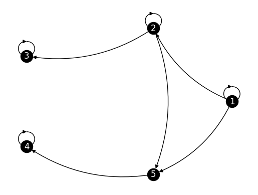
3 A Markov chain is irreducible if:
a) Every state communicates with every other state.
b) There exists a state that communicates with every other state.
c) The transition graph of the chain is strongly connected.
d) Both a and c.
4 Consider the following transition graph of a Markov chain:
G = nx.DiGraph()
G.add_edges_from([(1, 2), (2, 1), (2, 3), (3, 3)])
Is this Markov chain irreducible?
a) Yes
b) No
5 In an irreducible Markov chain, the left and right eigenvectors corresponding to eigenvalue 1 are:
a) The same up to scaling.
b) Always different.
c) Transposes of each other.
d) Not necessarily related to each other.
Answer for 1: b. Justification: The text states that a probability distribution \(\boldsymbol{\pi} = (\pi_i)_{i=1}^n\) over \([n]\) is a stationary distribution of a Markov chain with transition matrix \(P = (p_{i,j})_{i,j=1}^n\) if \(\sum_{i=1}^n \pi_i p_{i,j} = \pi_j\) for all \(j \in [n]\).
Answer for 2: a. Justification: The text states that the condition for a probability distribution \(\boldsymbol{\pi}\) to be a stationary distribution of a Markov chain with transition matrix \(P\) can be written in matrix form as \(\boldsymbol{\pi} P = \boldsymbol{\pi}\), where \(\boldsymbol{\pi}\) is thought of as a row vector.
Answer for 3: d. Justification: The text states that a Markov chain on \(S\) is irreducible if for all \(x, y \in S\) with \(x \neq y\), we have \(x \to y\) and \(y \to x\). It also mentions that a Markov chain is irreducible if and only if its transition graph is strongly connected.
Answer for 4: b. Justification: The Markov chain is not irreducible because there is no way to get back to state 1 from state 3.
Answer for 5: d. Justification: The text states that for an irreducible Markov chain, the left and right eigenvalues are the same, but the left and right eigenvectors are not necessarily the same. It also mentions that the geometric multiplicity of eigenvalue 1 is 1, implying that the left and right eigenvectors corresponding to eigenvalue 1 are unique up to scaling, but they are not necessarily related to each other.