
\(\newcommand{\bmu}{\boldsymbol{\mu}}\) \(\newcommand{\bSigma}{\boldsymbol{\Sigma}}\) \(\newcommand{\bfbeta}{\boldsymbol{\beta}}\) \(\newcommand{\bflambda}{\boldsymbol{\lambda}}\) \(\newcommand{\bgamma}{\boldsymbol{\gamma}}\) \(\newcommand{\bsigma}{{\boldsymbol{\sigma}}}\) \(\newcommand{\bpi}{\boldsymbol{\pi}}\) \(\newcommand{\btheta}{{\boldsymbol{\theta}}}\) \(\newcommand{\bphi}{\boldsymbol{\phi}}\) \(\newcommand{\balpha}{\boldsymbol{\alpha}}\) \(\newcommand{\blambda}{\boldsymbol{\lambda}}\) \(\renewcommand{\P}{\mathbb{P}}\) \(\newcommand{\E}{\mathbb{E}}\) \(\newcommand{\indep}{\perp\!\!\!\perp} \newcommand{\bx}{\mathbf{x}}\) \(\newcommand{\bp}{\mathbf{p}}\) \(\renewcommand{\bx}{\mathbf{x}}\) \(\newcommand{\bX}{\mathbf{X}}\) \(\newcommand{\by}{\mathbf{y}}\) \(\newcommand{\bY}{\mathbf{Y}}\) \(\newcommand{\bz}{\mathbf{z}}\) \(\newcommand{\bZ}{\mathbf{Z}}\) \(\newcommand{\bw}{\mathbf{w}}\) \(\newcommand{\bW}{\mathbf{W}}\) \(\newcommand{\bv}{\mathbf{v}}\) \(\newcommand{\bV}{\mathbf{V}}\) \(\newcommand{\bfg}{\mathbf{g}}\) \(\newcommand{\bfh}{\mathbf{h}}\) \(\newcommand{\horz}{\rule[.5ex]{2.5ex}{0.5pt}}\) \(\renewcommand{\S}{\mathcal{S}}\) \(\newcommand{\X}{\mathcal{X}}\) \(\newcommand{\var}{\mathrm{Var}}\) \(\newcommand{\pa}{\mathrm{pa}}\) \(\newcommand{\Z}{\mathcal{Z}}\) \(\newcommand{\bh}{\mathbf{h}}\) \(\newcommand{\bb}{\mathbf{b}}\) \(\newcommand{\bc}{\mathbf{c}}\) \(\newcommand{\cE}{\mathcal{E}}\) \(\newcommand{\cP}{\mathcal{P}}\) \(\newcommand{\bbeta}{\boldsymbol{\beta}}\) \(\newcommand{\bLambda}{\boldsymbol{\Lambda}}\) \(\newcommand{\cov}{\mathrm{Cov}}\) \(\newcommand{\bfk}{\mathbf{k}}\) \(\newcommand{\idx}[1]{}\) \(\newcommand{\xdi}{}\)
3.5. Gradient descent and its convergence analysis#
We consider a natural approach for solving optimization problems numerically: a class of algorithms known as descent methods.
Let \(f : \mathbb{R}^d \to \mathbb{R}\) be continuously differentiable. We restrict ourselves to unconstrained minimization problems of the form
Ideally one would like to identify a global minimizer of \(f\). A naive approach might be to evaluate \(f\) at a large number of points \(\mathbf{x}\), say on a dense grid. However, even if we were satisfied with an approximate solution and limited ourselves to a bounded subset of the domain of \(f\), this type of exhaustive search is wasteful and impractical in large dimension \(d\), as the number of points interrogated grows exponentially with \(d\).
A less naive approach might be to find all stationary points of \(f\), that is, those \(\mathbf{x}\) such that \(\nabla f(\mathbf{x}) = \mathbf{0}\). And then choose an \(\mathbf{x}\) among them that produces the smallest value of \(f(\mathbf{x})\). This indeed works in many problems, like the following example we have encountered previously.
EXAMPLE: (Least Squares) Consider again the least squares problem\(\idx{least squares problem}\xdi\)
where \(A \in \mathbb{R}^{n \times d}\) has full column rank and \(\mathbf{b} \in \mathbb{R}^n\). In particular, \(d \leq n\). We saw in a previous example that the objective function is a quadratic function
where \(P = 2 A^T A\) is symmetric, \(\mathbf{q} = - 2 A^T \mathbf{b}\), and \(r= \mathbf{b}^T \mathbf{b} = \|\mathbf{b}\|^2\). We also showed that \(f\) is \(\mu\)-strongly convex. So there is a unique global minimizer.
By a previous calculation,
So the stationary points satisfy
which you may recognize as the normal equations\(\idx{normal equations}\xdi\) for the least-squares problem. \(\lhd\)
Unfortunately, identifying stationary points often leads to systems of nonlinear equations that do not have explicit solutions. Hence we resort to a different approach.
3.5.1. Gradient descent#
In gradient descent, we attempt to find smaller values of \(f\) by successively following directions in which \(f\) decreases locally. As we have seen in the proof of the First-Order Necessary Optimality Condition, \(- \nabla f\) provides such a direction. In fact, it is the direction of steepest descent in the following sense.
Recall from the Descent Direction and Directional Derivative Lemma that \(\mathbf{v}\) is a descent direction at \(\mathbf{x}_0\) if the directional derivative of \(f\) at \(\mathbf{x}_0\) in the direction \(\mathbf{v}\) is negative.
LEMMA (Steepest Descent) \(\idx{steepest descent lemma}\xdi\) Let \(f : \mathbb{R}^d \to \mathbb{R}\) be continuously differentiable at \(\mathbf{x}_0\). For any unit vector \(\mathbf{v} \in \mathbb{R}^d\),
where
\(\flat\)
Proof idea: This is an immediate application of the Cauchy-Schwarz inequality.
Proof: By the Cauchy-Schwarz inequality, since \(\mathbf{v}\) has unit norm,
Or, put differently,
On the other hand, by the choice of \(\mathbf{v}^*\),
The last two displays combined give the result. \(\square\)
At each iteration of gradient descent, we take a step in the direction of the negative of the gradient, that is,
for a sequence of step sizes \(\alpha_t > 0\). Choosing the right step size (also known as steplength or learning rate) is a large subject in itself. We will only consider the case of fixed step size here.
CHAT & LEARN Ask your favorite AI chatbot about the different approaches for selecting a step size in gradient descent methods. \(\ddagger\)
In general, we will not be able to guarantee that a global minimizer is reached in the limit, even if one exists. Our goal for now is more modest: to find a point where the gradient of \(f\) approximately vanishes.
We implement gradient descent\(\idx{gradient descent}\xdi\) in Python. We assume that a function f and its gradient grad_f are provided. We first code the basic steepest descent step with a step size\(\idx{step size}\xdi\) \(\idx{learning rate}\xdi\) \(\alpha =\) alpha.
def desc_update(grad_f, x, alpha):
    return x - alpha*grad_f(x)

def gd(f, grad_f, x0, alpha=1e-3, niters=int(1e6)):

    xk = x0
    for _ in range(niters):
        xk = desc_update(grad_f, xk, alpha)

    return xk, f(xk)
NUMERICAL CORNER: We illustrate on a simple example.
def f(x):
    return (x-1)**2 + 10

def grad_f(x):
    return 2*(x-1)

xgrid = np.linspace(-5,5,100)
plt.plot(xgrid, f(xgrid), label='f')
plt.plot(xgrid, grad_f(xgrid), label='grad_f')
plt.ylim((-20,50)), plt.legend()
plt.show()
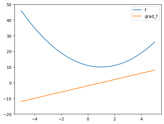
gd(f, grad_f, 0)
(0.9999999999999722, 10.0)
We found a global minmizer in this case.
The next example shows that a different local minimizer may be reached depending on the starting point.
def f(x):
    return 4 * (x-1)**2 * (x+1)**2 - 2*(x-1)

def grad_f(x):
    return 8 * (x-1) * (x+1)**2 + 8 * (x-1)**2 * (x+1) - 2

xgrid = np.linspace(-2,2,100)
plt.plot(xgrid, f(xgrid), label='f')
plt.plot(xgrid, grad_f(xgrid), label='grad_f')
plt.ylim((-10,10)), plt.legend()
plt.show()
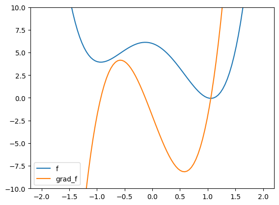
gd(f, grad_f, 0)
(1.057453770738375, -0.0590145651028224)
gd(f, grad_f, -2)
(-0.9304029265558538, 3.933005966859003)
TRY IT! In this last example, does changing the step size affect the outcome? (Open In Colab) \(\ddagger\)
In the final example, we end up at a stationary point that is not a local minimizer. Here both the first and second derivatives are zero. This is known as a saddle point.
def f(x):
    return x**3

def grad_f(x):
    return 3 * x**2

xgrid = np.linspace(-2,2,100)
plt.plot(xgrid, f(xgrid), label='f')
plt.plot(xgrid, grad_f(xgrid), label='grad_f')
plt.ylim((-10,10)), plt.legend()
plt.show()
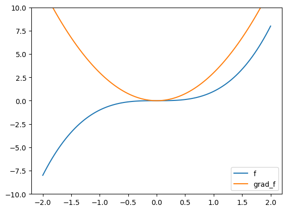
gd(f, grad_f, 2)
(0.00033327488712690107, 3.701755838398568e-11)
gd(f, grad_f, -2, niters=100)
(-4.93350410883896, -120.0788396909241)
\(\unlhd\)
3.5.2. Convergence analysis#
In this section, we prove some results about the convergence\(\idx{convergence analysis}\xdi\) of gradient descent. We start with the smooth case.
Smooth case Informally, a function is smooth if its gradient does not change too fast. The formal definition we will use here follows. We restrict ourselves to the twice continuously differentiable case.
DEFINITION (Smooth Function) \(\idx{smooth function}\xdi\) Let \(f : \mathbb{R}^d \to \mathbb{R}\) be twice continuously differentiable. We say that \(f\) is \(L\)-smooth if
\(\natural\)
In the single-variable case, this reduces to \(- L \leq f''(x) \leq L\) for all \(x \in \mathbb{R}\). More generally, recall that
So the condition above is equivalent to
A different way to put this is that the second directional derivative satisfies
for all \(\mathbf{x} \in \mathbb{R}^d\) and all unit vectors \(\mathbf{v} \in \mathbb{R}^d\).
Combined with Taylor’s Theorem, this gives immediately the following.
LEMMA (Quadratic Bound for Smooth Functions) \(\idx{quadratic bound for smooth functions}\xdi\) Let \(f : \mathbb{R}^d \to \mathbb{R}\) be twice continuously differentiable. Then \(f\) is \(L\)-smooth if and only if for all \(\mathbf{x}, \mathbf{y} \in \mathbb{R}^d\) it holds that
\(\flat\)
Proof idea: We apply the Taylor’s Theorem, then bound the second-order term.
Proof: By Taylor’s Theorem, for any \(\alpha > 0\) there is \(\xi_\alpha \in (0,1)\)
where \(\mathbf{p} = \mathbf{y} - \mathbf{x}\).
If \(f\) is \(L\)-smooth, then at \(\alpha = 1\) by the observation above
That implies the inequality in the statement.
On the other hand, if that inequality holds, by combining with the Taylor expansion above we get
where we used that \(\|\alpha \mathbf{p}\| = \alpha \|\mathbf{p}\|\) by absolute homogeneity of the norm. Dividing by \(\alpha^2/2\), then taking \(\alpha \to 0\) and using the continuity of the Hessian gives
By the observation above again, that implies that \(f\) is \(L\)-smooth. \(\square\)
We show next that, in the smooth case, steepest descent with an appropriately chosen step size produces a sequence of points whose objective values decrease (or stay the same) and whose gradients vanish in the limit. We also give a quantitative convergence rate. Note that this result does not imply convergence to a local (or global) minimizer.
THEOREM (Convergence of Gradient Descent in the Smooth Case) \(\idx{convergence of gradient descent in the smooth case}\xdi\) Suppose that \(f : \mathbb{R}^d \to \mathbb{R}\) is \(L\)-smooth and bounded from below, that is, there is \(\bar{f} > - \infty\) such that \(f(\mathbf{x}) \geq \bar{f}\), \(\forall \mathbf{x} \in \mathbb{R}^d\). Then gradient descent with step size \(\alpha_t = \alpha := 1/L\) started from any \(\mathbf{x}^0\) produces a sequence \(\mathbf{x}^t\), \(t=1,2,\ldots\) such that
and
Moreover, after \(S\) steps, there is a \(t\) in \(\{0,\ldots,S\}\) such that
\(\sharp\)
The assumption that a lower bound on \(f\) is known may seem far-fetched. But there are in fact many settings where this is natural. For instance, in the case of the least-squares problem, the objective function \(f\) is non-negative by definition and therefore we can take \(\bar{f} = 0\).
A different way to put the claim above regarding the convergence rate is the following. Take any \(\epsilon > 0\). If our goal is to find a point \(\mathbf{x}\) such that \(\|\nabla f(\mathbf{x})\| \leq \epsilon\), then we are guaranteed to find one if we perform \(S\) steps such that
that is, after rearranging,
The heart of the proof is the following fundamental inequality. It also informs the choice of step size.
LEMMA (Descent Guarantee in the Smooth Case) \(\idx{descent guarantee in the smooth case}\xdi\) Suppose that \(f : \mathbb{R}^d \to \mathbb{R}\) is \(L\)-smooth. For any \(\mathbf{x} \in \mathbb{R}^d\),
\(\flat\)
Proof idea (Descent Guarantee in the Smooth Case): Intuitively, the Quadratic Bound for Smooth Functions shows that \(f\) is well approximated by a quadratic function in a neighborhood of \(\mathbf{x}\) whose size depends on the smoothness parameter \(L\). Choosing a step size that minimizes this approximation leads to a guaranteed improvement. The approach taken here is a special case of what is referred to as Majorize-Minimization (MM)\(\idx{Majorize-Minimization}\xdi\).
Proof: (Descent Guarantee in the Smooth Case) By the Quadratic Bound for Smooth Functions, letting \(\mathbf{p} = - \nabla f(\mathbf{x})\)
The quadratic function in parentheses is convex and minimized at the stationary point \(\alpha\) satisfying
Taking \(\alpha = 1/L\), where \(-\alpha + \alpha^2 \frac{L}{2} = - \frac{1}{2L}\), and replacing in the inequality above gives
as claimed. \(\square\)
We return to the proof of the theorem.
Proof idea (Convergence of Gradient Descent in the Smooth Case): We use a telescoping argument to write \(f(\mathbf{x}^S)\) as a sum of stepwise increments, each of which can be bounded by the previous lemma. Because \(f(\mathbf{x}^S)\) is bounded from below, it then follows that the gradients must vanish in the limit.
Proof: (Convergence of Gradient Descent in the Smooth Case) By the Descent Guarantee in the Smooth Case,
Furthermore, using a telescoping sum, we get
Rearranging and using \(f(\mathbf{x}^S) \geq \bar{f}\) leads to
We get the quantitative bound
as the minimum is necessarily less or equal than the average. Moreover, as \(S \to +\infty\), we must have \(\|\nabla f(\mathbf{x}^S)\|^2 \to 0\) by standard analytical arguments. That proves the claim. \(\square\)
Smooth and strongly convex case With stronger assumptions, we obtain stronger convergence results. One such assumption is strong convexity, which we defined in the previous section for twice continuously differentiable functions.
We prove a convergence result for smooth, strongly convex functions. We show something stronger this time. We control the value of \(f\) itself and obtain a much faster rate of convergence. If \(f\) is \(m\)-strongly convex and has a global minimizer \(\mathbf{x}^*\), then the global minimizer is unique and characterized by \(\nabla f(\mathbf{x}^*) = \mathbf{0}\). Strong convexity allows us to relate the value of the function at a point \(\mathbf{x}\) and the gradient of \(f\) at that point. This is proved in the following lemma, which is key to our convergence result.
LEMMA (Relating a function and its gradient) \(\idx{relating a function and its gradient lemma}\xdi\) Let \(f : \mathbb{R}^d \to \mathbb{R}\) be twice continuously differentiable, \(m\)-strongly convex with a global minimizer at \(\mathbf{x}^*\). Then for any \(\mathbf{x} \in \mathbb{R}^d\)
\(\flat\)
Proof: By the Quadratic Bound for Strongly Convex Functions,
where on the second line we defined \(\mathbf{w} = \mathbf{x}^* - \mathbf{x}\). The right-hand side is a quadratic function in \(\mathbf{w}\) (for \(\mathbf{x}\) fixed), and on the third line we used our previous notation \(P\), \(\mathbf{q}\) and \(r\) for such a function. So the inequality is still valid if we replace \(\mathbf{w}\) with the global minimizer \(\mathbf{w}^*\) of that quadratic function.
The matrix \(P = m I_{d \times d}\) is positive definite. By a previous example, we know that the minimizer is achieved when the gradient \(\frac{1}{2}[P + P^T]\mathbf{w}^* + \mathbf{q} = \mathbf{0}\), which is equivalent to
So, replacing \(\mathbf{w}\) with \(\mathbf{w}^*\), we have the inequality
Rearranging gives the claim. \(\square\)
We can now state our convergence result.
THEOREM (Convergence of Gradient Descent in the Strongly Convex Case) \(\idx{convergence of gradient descent in the strongly convex case}\xdi\) Suppose that \(f : \mathbb{R}^d \to \mathbb{R}\) is \(L\)-smooth and \(m\)-strongly convex with a global minimizer at \(\mathbf{x}^*\). Then gradient descent with step size \(\alpha = 1/L\) started from any \(\mathbf{x}^0\) produces a sequence \(\mathbf{x}^t\), \(t=1,2,\ldots\) such that
Moreover, after \(S\) steps, we have
\(\sharp\)
Observe that \(f(\mathbf{x}^S) - f(\mathbf{x}^*)\) decreases exponentially fast in \(S\). A related bound can be proved for \(\|\mathbf{x}^S - \mathbf{x}^*\|\).
Put differently, fix any \(\epsilon > 0\). If our goal is to find a point \(\mathbf{x}\) such that \(f(\mathbf{x}) - f(\mathbf{x}^*) \leq \epsilon\), then we are guaranteed to find one if we perform \(S\) steps such that
that is, after rearranging,
Proof idea (Convergence of Gradient Descent in the Strongly Convex Case): We apply the Descent Guarantee for Smooth Functions together with the lemma above.
Proof: (Convergence of Gradient Descent in the Strongly Convex Case) By the Descent Guarantee for Smooth Functions together with the lemma above, we have for all \(t\)
Subtracting \(f(\mathbf{x}^*)\) on both sides gives
Recursing this is
and so on. That gives the claim. \(\square\)
NUMERICAL CORNER: We revisit our first simple single-variable example.
def f(x):
    return (x-1)**2 + 10

def grad_f(x):
    return 2*(x-1)
The second derivative is \(f''(x) = 2\). Hence, this \(f\) is \(L\)-smooth and \(m\)-strongly convex with \(L = m = 2\). The theory we developed suggests taking step size \(\alpha_t = \alpha = 1/L = 1/2\). It also implies that
We converge in one step! And that holds for any starting point \(x^0\).
Let’s try this!
gd(f, grad_f, 0, alpha=0.5, niters=1)
(1.0, 10.0)
Let’s try a different starting point.
gd(f, grad_f, 100, alpha=0.5, niters=1)
(1.0, 10.0)
\(\unlhd\)
Self-assessment quiz (with help from Claude, Gemini, and ChatGPT)
1 In the gradient descent update rule \(\mathbf{x}^{t+1} = \mathbf{x}^t - \alpha_t \nabla f(\mathbf{x}^t)\), what does \(\alpha_t\) represent?
a) The gradient of \(f\) at \(\mathbf{x}^t\)
b) The step size or learning rate
c) The direction of steepest ascent
d) The Hessian matrix of \(f\) at \(\mathbf{x}^t\)
2 A function \(f : \mathbb{R}^d \to \mathbb{R}\) is said to be \(L\)-smooth if:
a) \(\|\nabla f(\mathbf{x})\| \leq L\) for all \(\mathbf{x} \in \mathbb{R}^d\)
b) \(-LI_{d\times d} \preceq \mathbf{H}_f(\mathbf{x}) \preceq LI_{d\times d}\) for all \(\mathbf{x} \in \mathbb{R}^d\)
c) \(f(\mathbf{y}) \leq f(\mathbf{x}) + \nabla f(\mathbf{x})^T(\mathbf{y} - \mathbf{x}) + \frac{L}{2}\|\mathbf{y} - \mathbf{x}\|^2\) for all \(\mathbf{x}, \mathbf{y} \in \mathbb{R}^d\)
d) Both b) and c)
3 Suppose \(f : \mathbb{R}^d \to \mathbb{R}\) is \(L\)-smooth and bounded from below. According to the Convergence of Gradient Descent in the Smooth Case theorem, gradient descent with step size \(\alpha_t = 1/L\) started from any \(\mathbf{x}^0\) produces a sequence \(\{\mathbf{x}^t\}\) such that
a) \(\lim_{t \to +\infty} f(\mathbf{x}^t) = 0\)
b) \(\lim_{t \to +\infty} \|\nabla f(\mathbf{x}^t)\| = 0\)
c) \(\min_{t=0,\ldots,S-1} \|\nabla f(\mathbf{x}^t)\| \leq \sqrt{\frac{2L[f(\mathbf{x}^0) - \bar{f}]}{S}}\) after \(S\) steps
d) Both b) and c)
4 Suppose \(f : \mathbb{R}^d \to \mathbb{R}\) is \(L\)-smooth and \(m\)-strongly convex with a global minimizer at \(\mathbf{x}^*\). According to the Convergence of Gradient Descent in th Strongly Convex Case theorem, gradient descent with step size \(\alpha = 1/L\) started from any \(\mathbf{x}^0\) produces a sequence \(\{\mathbf{x}^t\}\) such that after \(S\) steps:
a) \(f(\mathbf{x}^S) - f(\mathbf{x}^*) \leq (1 - \frac{m}{L})^S[f(\mathbf{x}^0) - f(\mathbf{x}^*)]\)
b) \(f(\mathbf{x}^S) - f(\mathbf{x}^*) \geq (1 - \frac{m}{L})^S[f(\mathbf{x}^0) - f(\mathbf{x}^*)]\)
c) \(f(\mathbf{x}^S) - f(\mathbf{x}^*) \leq (1 + \frac{m}{L})^S[f(\mathbf{x}^0) - f(\mathbf{x}^*)]\)
d) \(f(\mathbf{x}^S) - f(\mathbf{x}^*) \geq (1 + \frac{m}{L})^S[f(\mathbf{x}^0) - f(\mathbf{x}^*)]\)
5 If a function \(f\) is \(m\)-strongly convex, what can we say about its global minimizer?
a) It may not exist.
b) It exists and is unique.
c) It exists but may not be unique.
d) It always occurs at the origin.
Answer for 1: b. Justification: The text states “At each iteration of gradient descent, we take a step in the direction of the negative of the gradient, that is, \(\mathbf{x}^{t+1} = \mathbf{x}^t - \alpha_t \nabla f(\mathbf{x}^t), t = 0, 1, 2, \ldots\) for a sequence of step sizes \(\alpha_t > 0\).”
Answer for 2: d. Justification: The text provides both the definition in terms of the Hessian matrix (option b) and the equivalent characterization in terms of the quadratic bound (option c).
Answer for 3: d. Justification: The theorem states both the asymptotic convergence of the gradients to zero (option b) and the quantitative bound on the minimum gradient norm after \(S\) steps (option c).
Answer for 4: a. Justification: This is the convergence rate stated in the theorem.
Answer for 5: b. Justification: The text states that if \(f\) is \(m\)-strongly convex, then “the global minimizer is unique.”