7.8.1.1. Just the code#

An interactive Jupyter notebook featuring the code in this chapter can be accessed below (Google Colab recommended). You are encouraged to tinker with it. Some suggested computational exercises are scattered throughout. The notebook is also available as a slideshow.

• Notebook (Open In Colab)

• Slideshow

7.8.1.2. Self-assessment quizzes#

A more extensive web version of the self-assessment quizzes is available by following the links below.

• Section 7.2

• Section 7.3

• Section 7.4

• Section 7.5

• Section 7.6

7.8.1.3. Auto-quizzes#

Automatically generated quizzes for this chapter can be accessed here (Google Colab recommended).

• Auto-quizzes (Open In Colab)

7.8.1.4. Solutions to odd-numbered warm-up exercises#

(with help from Claude, Gemini, and ChatGPT)

E7.2.1 We need to check that all entries of $P$ are non-negative and that all rows sum to one.

Non-negativity: All entries of $P$ are clearly non-negative.

Row sums: Row 1: $0.2+0.5+0.3=1$ Row 2: $0.4+0.1+0.5=1$ Row 3: $0.6+0.3+0.1=1$

Therefore, $P$ is a stochastic matrix.

E7.2.3

E7.2.5

G = nx.DiGraph()
G.add_nodes_from(range(1, 5))
G.add_edges_from([(1, 2), (1, 4), (2, 1), (2, 3), (3, 2), (3, 4), (4, 1), (4, 3)])

The transition graph has a directed edge from state $i$ to state $j$ if and only if $p_{i,j}>0$, as stated in the definition.

E7.2.7

E7.2.9 The probability is given by the entry $(P^2{)}_{0,1}$, where $P^2$ is the matrix product $P\times P$.

Therefore, the probability is $\boxed{{\displaystyle 11/18}}$.

E7.2.11 The marginal distribution at time 2 is given by $\mu P^2$.

Thus,

E7.2.13 The distribution at time 1 is given by $\mu P$.

E7.2.15 The chain alternates deterministically between states 1 and 2. Therefore, starting in state 1, it will return to state 1 after exactly $\boxed{{\displaystyle 2}}$ steps.

E7.3.1 Yes, the matrix is irreducible. The corresponding transition graph is a cycle, which is strongly connected.

E7.3.3 We need to check if $\pi P=\pi$. Indeed,

so $\pi$ is not a stationary distribution of the Markov chain.

E7.3.5 Let $\pi =({\pi }_1,{\pi }_2)$ be a stationary distribution. Then, we need to solve the system of equations:

The first equation simplifies to ${\pi }_1={\pi }_2$, and substituting this into the second equation yields $2{\pi }_1=1$, or ${\pi }_1={\pi }_2=0.5$. Therefore, $\pi =(0.5,0.5)$ is a stationary distribution.

E7.3.7 To verify that $\pi$ is a stationary distribution, we need to check if $\pi P=\pi$. Let’s perform the matrix multiplication step by step:

$\pi P=(\frac{1}{3},\frac{1}{3},\frac{1}{3})\left(\begin{array}{ccc}0.4& 0.3& 0.3\\ 0.2& 0.5& 0.3\\ 0.4& 0.2& 0.4\end{array}\right)$

$=(\frac{1}{3}\cdot 0.4+\frac{1}{3}\cdot 0.2+\frac{1}{3}\cdot 0.4,\frac{1}{3}\cdot 0.3+\frac{1}{3}\cdot 0.5+\frac{1}{3}\cdot 0.2,\frac{1}{3}\cdot 0.3+\frac{1}{3}\cdot 0.3+\frac{1}{3}\cdot 0.4)$

$=(\frac{0.4+0.2+0.4}{3},\frac{0.3+0.5+0.2}{3},\frac{0.3+0.3+0.4}{3})$

$=(\frac{1}{3},\frac{1}{3},\frac{1}{3})$

$=\pi$

The result is equal to $\pi =(\frac{1}{3},\frac{1}{3},\frac{1}{3})$. Therefore, the uniform distribution $\pi$ is indeed a stationary distribution for the matrix $P$. Note that the transition matrix $P$ is doubly stochastic because each row and each column sums to 1. This property ensures that the uniform distribution is always a stationary distribution for doubly stochastic matrices, as mentioned in the text.

E7.3.9 Let $\mathbf{1}=(1,1,\dots ,1{)}^T$ be the column vector of all ones. For any stochastic matrix $P$, we have:

because each row of a stochastic matrix sums to 1. Therefore, $\mathbf{1}$ is a right eigenvector of $P$ with eigenvalue 1.

E7.3.11 Let $\pi =({\pi }_1,{\pi }_2,{\pi }_3)$ be the stationary distribution. We need to solve the system of equations:

Step 1: Write out the system of equations based on $\pi P=\pi$.

Step 2: Rearrange the equations to have zero on the right-hand side.

Step 3: Simplify the equations.

Step 4: Use the condition ${\pi }_1+{\pi }_2+{\pi }_3=1$ to eliminate one variable, say ${\pi }_3$.

Step 5: Substitute the expression for ${\pi }_3$ into the simplified equations from Step 3.

Step 6: Simplify the equations further.

Step 7: Solve the linear system of two equations with two unknowns using any suitable method (e.g., substitution, elimination, or matrix inversion).

Using the substitution method: From the second equation, express ${\pi }_1$ in terms of ${\pi }_2$:

Substitute this into the first equation:

Now, substitute ${\pi }_2=\frac{3}{13}$ back into the expression for ${\pi }_1$:

Finally, use ${\pi }_1+{\pi }_2+{\pi }_3=1$ to find ${\pi }_3$:

Therefore, the stationary distribution is $(\frac{8}{13},\frac{3}{13},\frac{2}{13})$.

E7.4.1 Given the transition matrix of a Markov chain:

determine if the chain is lazy.

E7.4.3 Given a Markov chain with transition matrix:

and initial distribution $\mu =(0.2,0.8)$, compute $\underset{t\to \mathrm{\infty }}{lim}\mu P^t$.

E7.5.1 The degree matrix $D$ is

The degrees are computed by summing the entries in each row of $A$.

E7.5.3 A stochastic matrix has rows that sum to 1. The rows of $P$ sum to 1:

Thus, $P$ is stochastic.

E7.5.5

E7.5.7 First, compute the transition matrix:

Then, compute the modified transition matrix with the damping factor:

E7.5.9 First, compute the transition matrix:

Then, compute the modified transition matrix with the damping factor:

E7.5.11 The new adjacency matrix $A^{\prime }$ is

A self-loop is added to vertex 4.

E7.5.13 The modified transition matrix $Q$ is

Using the values from $P$ and ${11}^T$, we get:

E7.6.1 The acceptance probability is given by

E7.6.3 Since the proposal chain is symmetric, the acceptance probability simplifies to $$min\{1,\frac{{\pi }_2}{{\pi }_1}\}=min\{1,\frac{0.2}{0.1}\}=1.$$

E7.6.5 The acceptance probability is given by

E7.6.7 The conditional probability is given by

E7.6.9 The energy is given by

E7.6.11 The conditional mean for the hidden units is:

For $h_1$:

For $h_2$:

7.8.1.5. Learning outcomes#

• Define a discrete-time Markov chain and its state space, initial distribution, and transition probabilities.

• Identify Markov chains in real-world scenarios, such as weather patterns or random walks on graphs.

• Construct the transition matrix for a time-homogeneous Markov chain.

• Construct the transition graph of a Markov chain from its transition matrix.

• Prove that the transition matrix of a Markov chain is a stochastic matrix.

• Apply the Markov property to calculate the probability of specific sequences of events in a Markov chain using the distribution of a sample path.

• Compute the marginal distribution of a Markov chain at a specific time using matrix powers.

• Use simulation to generate sample paths of a Markov chain.

• Define a stationary distribution of a finite-state, discrete-time, time-homogeneous Markov chain and express the defining condition in matrix form.

• Explain the relationship between stationary distributions and left eigenvectors of the transition matrix.

• Determine whether a given probability distribution is a stationary distribution for a given Markov chain.

• Identify irreducible Markov chains and explain their significance in the context of stationary distributions.

• State the main theorem on the existence and uniqueness of a stationary distribution for an irreducible Markov chain.

• Compute the stationary distribution of a Markov chain numerically using either eigenvalue methods or by solving a linear system of equations, including the “Replace an Equation” method.

• Define the concepts of aperiodicity and weak laziness for finite-space discrete-time Markov chains.

• State the Convergence to Equilibrium Theorem and the Ergodic Theorem for irreducible Markov chains.

• Verify the Ergodic Theorem by simulating a Markov chain and comparing the frequency of visits to each state with the stationary distribution.

• Explain the concept of coupling and its role in proving the Convergence to Equilibrium Theorem for irreducible, weakly lazy Markov chains.

• Define random walks on directed and undirected graphs, and express their transition matrices in terms of the adjacency matrix.

• Determine the stationary distribution of a random walk on an undirected graph and explain its relation to degree centrality.

• Explain the concept of reversibility and its connection to the stationary distribution of a random walk.

• Describe the PageRank algorithm and its interpretation as a modified random walk on a directed graph.

• Compute the PageRank vector by finding the stationary distribution of the modified random walk using power iteration.

• Apply the PageRank algorithm to real-world datasets to identify central nodes in a network.

• Explain the concept of Personalized PageRank and how it differs from the standard PageRank algorithm.

• Modify the PageRank algorithm to implement Personalized PageRank and interpret the results based on the chosen teleportation distribution.

• Describe the concept of Markov Chain Monte Carlo (MCMC) and its application in sampling from complex probability distributions.

• Explain the Metropolis-Hastings algorithm, including the proposal distribution and acceptance-rejection steps.

• Calculate acceptance probabilities in the Metropolis-Hastings algorithm for a given target and proposal distribution.

• Prove the correctness of the Metropolis-Hastings algorithm by showing that the resulting Markov chain is irreducible and reversible with respect to the target distribution.

• Implement the Gibbs sampling algorithm for a given probabilistic model, such as a Restricted Boltzmann Machine (RBM).

• Analyze the conditional independence properties of RBMs and their role in Gibbs sampling.

$\mathrm{\aleph }$

7.8.2.1. Random walk on a weighted graph#

The previous definitions extend naturally to the weighted case. Again we allow loops, i.e., self-weights $w_{i,i}>0$. For a weighted graph $G$, recall that the degree of a vertex is defined as

which includes the self-weight $w_{i,i}$, and where we use the convention that $w_{i,j}=0$ if $\{i,j\}\notin E$. Recall also that $w_{i,j}=w_{j,i}$.

DEFINITION (Random Walk on a Weighted Graph) Let $G=(V,E,w)$ be a weighted graph with positive edge weights. Assume all vertices have a positive degree. A random walk on $G$ is a time-homogeneous Markov chain $(X_t{)}_{t\ge 0}$ with state space $\mathcal{S}=V$ and transition probabilities

$\mathrm{♮}$

Once again, it is easily seen that the transition matrix of random walk on $G$ satisfying the conditions of the definition above is $P=D^{-1}A,$ where $D=\mathrm{diag}(A\mathbf{1})$ is the degree matrix.

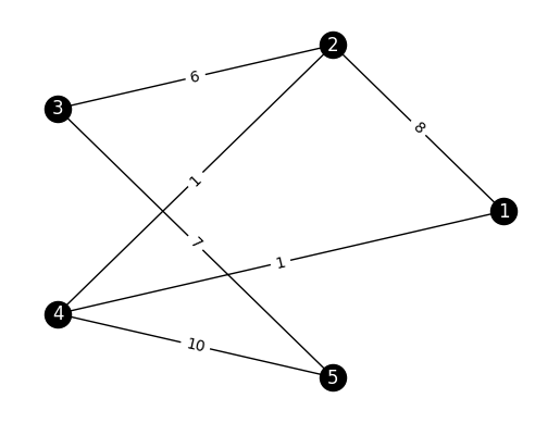
EXAMPLE: (A Weighted Graph) Here is another example. Consider the following adjacency matrix on $5$ vertices.

A_ex = np.array([
    [0, 8, 0, 1, 0],
    [8, 0, 6, 1, 0],
    [0, 6, 0, 0, 7],
    [1, 1, 0, 0, 10],
    [0, 0, 7, 10, 0]])

It is indeed a symmetric matrix.

print(LA.norm(A_ex.T - A_ex))

0.0

We define a graph from its adjacency matrix.

n_ex = A_ex.shape[0] # number of vertices
G_ex = nx.from_numpy_array(A_ex) # graph

To draw it, we first define edge labels by creating a dictionary that assigns to each edge (as a tuple) its weight. Here G.edges.data('weight') (see G.edges) iterates through the edges (u,v) and includes their weight as the third entry of the tuple (u,v,w). Then we use the function networkx.draw_networkx_edge_labels() to add the weights as edge labels.

edge_labels = {}
for (u,v,w) in G_ex.edges.data('weight'):
    edge_labels[(u,v)] = w

pos=nx.circular_layout(G_ex)
nx.draw_networkx(G_ex, pos, labels={i: i+1 for i in range(n_ex)},
                 node_color='black', font_color='white')
edge_labels = nx.draw_networkx_edge_labels(G_ex, pos, edge_labels=edge_labels)
plt.axis('off')
plt.show()

The transition matrix of the random walk on this graph can be computed using the lemma above. We first compute the degree matrix, then apply the formula.

degrees_ex = A_ex @ np.ones(n_ex)
inv_degrees_ex = 1/ degrees_ex
Dinv_ex = np.diag(inv_degrees_ex)
P_ex = Dinv_ex @ A_ex
print(P_ex)

[[0.         0.88888889 0.         0.11111111 0.        ]
 [0.53333333 0.         0.4        0.06666667 0.        ]
 [0.         0.46153846 0.         0.         0.53846154]
 [0.08333333 0.08333333 0.         0.         0.83333333]
 [0.         0.         0.41176471 0.58823529 0.        ]]

This is indeed a stochastic matrix.

print(P_ex @ np.ones(n_ex))

[1. 1. 1. 1. 1.]

$⊲$

LEMMA (Irreducibility in Undirected Case) Let $G=(V,E,w)$ be a graph with positive edge weights. Assume all vertices have a positive degree. Random walk on $G$ is irreducible if and only if $G$ is connected. $\mathrm{♭}$

THEOREM (Stationary Distribution on a Graph) Let $G=(V,E,w)$ be a graph with positive edge weights. Assume further that $G$ is connected. Then the unique stationary distribution of random walk on $G$ is given by

$\mathrm{♯}$

EXAMPLE: (A Weighted Graph, continued) Going back to our weighted graph example, we use the previous theorem to compute the stationary distribution. Note that the graph is indeed connected so the stationary distribution is unique. We have already computed the degrees.

print(degrees_ex)

[ 9. 15. 13. 12. 17.]

We compute $\sum _{i\in V}\delta (i)$ next.

total_degrees_ex = degrees_ex @ np.ones(n_ex)
print(total_degrees_ex)

66.0

Finally, the stationary distribution is:

pi_ex = degrees_ex / total_degrees_ex
print(pi_ex)

[0.13636364 0.22727273 0.1969697  0.18181818 0.25757576]

We check stationarity.

print(LA.norm(P_ex.T @ pi_ex - pi_ex))

2.7755575615628914e-17

$⊲$

A random walk on a weighted undirected graph is reversible. Vice versa, it turns out that any reversible chain can be seen as a random walk on an appropriately defined weighted undirected graph. See the exercises.

7.8.2.2. Spectral techniques for random walks on graphs#

In this section, we use techniques from spectral graph theory to analyze random walks on graphs.

Applying the spectral theorem via the normalized Laplacian We have seen how to compute the unique stationary distribution $\mathit{\pi }$ of random walk on a connected weighted (undirected) graph. Recall that $\mathit{\pi }$ is a (left) eigenvector of $P$ with eigenvalue $1$ (i.e., $\mathit{\pi }P=\mathit{\pi }$). In general, however, the matrix $P$ is not symmetric in this case (see the previous example) - even though the adjacency matrix is. So we cannot apply the spectral theorem to get the rest of the eigenvectors - if they even exist. But, remarkably, a symmetric matrix with the a closely related spectral decomposition is hiding in the background.

Recall that the normalized Laplacian of a weighted graph $G=(V,E,w)$ with adjacency matrix $A$ and degree matrix $D$ is defined as

Recall that in the weighted case, the degree is defined as $\delta (i)=\sum _{j:\{i,j\}\in E}{w}_{i,j}$. Because it is symmetric and positive semi-definite, we can write

where the ${\mathbf{z}}_i$s are orthonormal eigenvectors of $\mathcal{L}$ and the eigenvalues satisfy $0\le {\eta }_1\le {\eta }_2\le \cdots \le {\eta }_n$.

Moreover, $D^{1/2}\mathbf{1}$ is an eigenvector of $\mathcal{L}$ with eigenvalue $0$. So ${\eta }_1=0$ and we set

which makes ${\mathbf{z}}_1$ into a unit norm vector.

We return to the eigenvectors of $P$. When a matrix $A\in {\mathbb{R}}^{n\times n}$ is diagonalizable, it has an eigendecomposition of the form

where $\mathrm{\Lambda }$ is a diagonal matrix whose diagonal entries are the eigenvalues of $A$. The columns of $Q$ are the eigenvectors of $A$ and they form a basis of ${\mathbb{R}}^n$. Unlike the symmetric case, however, the eigenvectors need not be orthogonal.

THEOREM (Eigendecomposition of Random Walk on a Graph) Let $G=(V,E,w)$ be a graph with positive edge weights and no isolated vertex, and with degree matrix $D$. Let $P\in {\mathbb{R}}^{n\times n}$ be the transition matrix of random walk on $G$. Let ${\mathbf{z}}_1,\dots ,{\mathbf{z}}_n\in {\mathbb{R}}^n$ and $0\le {\eta }_1\le \cdots {\eta }_n\le 2$ be the eigenvectors and eigenvalues of the normalized Laplacian. Then $P$ has the following eigendecomposition

where the columns of $Z$ are the ${\mathbf{z}}_i$s and $H$ is a diagonal matrix with the ${\eta }_i$s on its diagonal. This can also be written as

where

$\mathrm{♯}$

Proof: We write $\mathcal{L}$ in terms of $P$. Recall that $P=D^{-1}A$. Hence

Rearranging this becomes

Hence for all $i=1,\dots ,n$

Because $P$ is a transition matrix, all its eigenvalues are bounded in absolute value by $1$. So $|1-{\eta }_i|\le 1$, which implies $0\le {\eta }_i\le 2$.

We also note that

by the orthonormality of the eigenvectors of the normalized Laplacian. So the columns of $D^{-1/2}Z$, i.e, $D^{-1/2}{\mathbf{z}}_i$ for $i=1,\dots ,n$, are linearly independent and

That gives the first claim.

To get the second claim, we first note that (for similar calculations, see the definition of an SVD)

where ${\lambda }_i=1-{\eta }_i$.

We then use the expression for ${\mathbf{z}}_1$ above. We have

while

So

That proves the second claim. $◻$

If $G$ is connected and $w_{i,i}>0$ for all $i$, then the chain is irreducible and lazy. In that case, there is a unique eigenvalue $1$ and $-1$ is not an eigenvalue, so we must have $0<{\eta }_2\le \cdots \le {\eta }_n<2$.

Limit theorems revisited The Convergence to Equilibrium Theorem implies that in the irreducible, aperiodic case

as $t\to +\mathrm{\infty }$, for any initial distribution $\mathit{\mu }$ and the unique stationary distribution $\mathit{\pi }$. Here we give a simpler proof for random walk on a graph (or more generally a reversible chain), with the added bonus of a convergence rate. This follows from the same argument we used in the Power Iteration Lemma.

DEFINITION (Spectral Gap) Let $G=(V,E,w)$ be a graph with positive edge weights and no isolated vertex. Let $P\in {\mathbb{R}}^{n\times n}$ be the transition matrix of random walk on $G$. The absolute spectral gap of $G$ is defined as ${\gamma }_{\star }=1-{\lambda }_{\star }$ where

$\mathrm{♮}$

THEOREM (Convergence to Equilibrium: Reversible Case) Let $G=(V,E,w)$ be a connected graph with positive edge weights and $w_{x,x}>0$ for all $x\in V$. Let $P\in {\mathbb{R}}^{n\times n}$ be the transition matrix of random walk on $G$ and $\mathit{\pi }$ its unique stationary distribution. Then

as $t\to +\mathrm{\infty }$ for any initial distribution $\mathit{\mu }$. Moreover,

where $\overline{\delta }=\underset{x}{max}\delta (x)$, $\underset{―}{\delta }=\underset{x}{min}\delta (x)$ and ${\gamma }_{\star }$ is the absolute spectral gap. $\mathrm{♯}$

Proof: Similarly to the Power Iteration Lemma, using the Eigendecomposition of Random Walk on a Graph we get

By induction,

by calculations similar to the proof of the Eigendecomposition of Random Walk on a Graph.

In the irreducible, lazy case, for $i=2,\dots ,n$, ${\lambda }_i^t\to 0$ as $t\to +\mathrm{\infty }$.

Moreover, $|{\lambda }_i|\le (1-{\gamma }_{\star })$ for all $i=2,\dots ,n$. Hence,

We then use Cauchy-Schwarz and the fact that $Z{Z}^T=I$ (as $Z$ is an orthogonal matrix), which implies $\sum _{i=1}^n({\mathbf{z}}_i{)}_x^2=1$.

We get that the above is

$◻$

We record an immediate corollary that will be useful next. Let $f:V\to \mathbb{R}$ be a function over the vertices. Define the (column) vector $\mathbf{f}=(f(1),\dots ,f(n){)}^T$ and note that

It will be convenient to use to ${\ell }_{\mathrm{\infty }}$-norm. For a vector $\mathbf{x}=(x_1,\dots ,x_n{)}^T$, we let $\Vert \mathbf{x}{\Vert }_{\mathrm{\infty }}=\underset{i\in [n]}{max}|x_i|$.

THEOREM For any initial distribution $\mathit{\mu }$ and any $t$

$\mathrm{♯}$

Proof: By the Time Marginals Theorem,

Because $\sum _x{\mu }_x=1$, the right-hand side is

by the triangle inequality.

Now by the theorem this is

That proves the claim. $◻$

We also prove a version of the Ergodic Theorem.

THEOREM (Ergodic Theorem: Reversible Case) Let $G=(V,E,w)$ be a connected graph with positive edge weights and $w_{x,x}>0$ for all $x\in V$. Let $P\in {\mathbb{R}}^{n\times n}$ be the transition matrix of random walk on $G$ and $\mathit{\pi }$ its unique stationary distribution. Let $f:V\to \mathbb{R}$ be a function over the vertices. Then for any initial distribution $\mathit{\mu }$

in probability as $T\to +\mathrm{\infty }$. $\mathrm{♯}$

Proof idea: We use Chebyshev’s Inequality. By the Convergence Theorem: Reversible Case, the expectation converges to the limit. To bound the variance, we use the Eigendecomposition of Random Walk on a Graph.

Proof: We use Chebyshev’s Inequality, similarly to our proof of the Weak Law of Large Numbers. However, unlike that case, here the terms in the sum are not independent are require some finessing. Define again the (column) vector $\mathbf{f}=(f(1),\dots ,f(n))$. Then the limit can be written as

By the corollary, the expectation of the sum can be bounded as follows

as $T\to +\mathrm{\infty }$.

Next we bound the variance of the sum. By the Variance of a Sum,