
\(\newcommand{\bmu}{\boldsymbol{\mu}}\) \(\newcommand{\bSigma}{\boldsymbol{\Sigma}}\) \(\newcommand{\bfbeta}{\boldsymbol{\beta}}\) \(\newcommand{\bflambda}{\boldsymbol{\lambda}}\) \(\newcommand{\bgamma}{\boldsymbol{\gamma}}\) \(\newcommand{\bsigma}{{\boldsymbol{\sigma}}}\) \(\newcommand{\bpi}{\boldsymbol{\pi}}\) \(\newcommand{\btheta}{{\boldsymbol{\theta}}}\) \(\newcommand{\bphi}{\boldsymbol{\phi}}\) \(\newcommand{\balpha}{\boldsymbol{\alpha}}\) \(\newcommand{\blambda}{\boldsymbol{\lambda}}\) \(\renewcommand{\P}{\mathbb{P}}\) \(\newcommand{\E}{\mathbb{E}}\) \(\newcommand{\indep}{\perp\!\!\!\perp} \newcommand{\bx}{\mathbf{x}}\) \(\newcommand{\bp}{\mathbf{p}}\) \(\renewcommand{\bx}{\mathbf{x}}\) \(\newcommand{\bX}{\mathbf{X}}\) \(\newcommand{\by}{\mathbf{y}}\) \(\newcommand{\bY}{\mathbf{Y}}\) \(\newcommand{\bz}{\mathbf{z}}\) \(\newcommand{\bZ}{\mathbf{Z}}\) \(\newcommand{\bw}{\mathbf{w}}\) \(\newcommand{\bW}{\mathbf{W}}\) \(\newcommand{\bv}{\mathbf{v}}\) \(\newcommand{\bV}{\mathbf{V}}\) \(\newcommand{\bfg}{\mathbf{g}}\) \(\newcommand{\bfh}{\mathbf{h}}\) \(\newcommand{\horz}{\rule[.5ex]{2.5ex}{0.5pt}}\) \(\renewcommand{\S}{\mathcal{S}}\) \(\newcommand{\X}{\mathcal{X}}\) \(\newcommand{\var}{\mathrm{Var}}\) \(\newcommand{\pa}{\mathrm{pa}}\) \(\newcommand{\Z}{\mathcal{Z}}\) \(\newcommand{\bh}{\mathbf{h}}\) \(\newcommand{\bb}{\mathbf{b}}\) \(\newcommand{\bc}{\mathbf{c}}\) \(\newcommand{\cE}{\mathcal{E}}\) \(\newcommand{\cP}{\mathcal{P}}\) \(\newcommand{\bbeta}{\boldsymbol{\beta}}\) \(\newcommand{\bLambda}{\boldsymbol{\Lambda}}\) \(\newcommand{\cov}{\mathrm{Cov}}\) \(\newcommand{\bfk}{\mathbf{k}}\) \(\newcommand{\idx}[1]{}\) \(\newcommand{\xdi}{}\)
4.4. Power iteration#
There is in general no exact method for computing SVDs. Instead we must rely on iterative methods, that is, methods that progressively approach the solution. We describe in this section the power iteration method. This method is behind an effective numerical approach for computing SVDs.
The focus here is on numerical methods and we will not spend much time computing SVDs by hand. But note that the connection between the SVD and the spectral decomposition of \(A^T A\) can be used for this purpose on small examples.
4.4.1. Key lemma#
We now derive the main idea behind an algorithm to compute singular vectors. Let \(U \Sigma V^T\) be a (compact) SVD of \(A\). Because of the orthogonality of \(U\) and \(V\), the powers of \(A^T A\) have a simple representation. Indeed
Note that this formula is closely related to our previously uncovered connection between the SVD and the spectral decomposition of \(A^T A\) – although it is not quite a spectral decomposition of \(A^T A\) since \(V\) is not orthogonal.
Iterating,
and, for general \(k\),
Hence, defining
we see that
When \(\sigma_1 > \sigma_2, \ldots, \sigma_r\), which is typically the case with real datasets, we get that \(\sigma_1^{2k} \gg \sigma_2^{2k}, \ldots, \sigma_r^{2k}\) when \(k\) is large. Then, we get the approximation
Finally, we arrive at:
LEMMA (Power Iteration) \(\idx{power iteration lemma}\xdi\) Let \(A \in \mathbb{R}^{n\times m}\) be a matrix and let \(U \Sigma V^T\) be a (compact) SVD of \(A\) such that \(\sigma_1 > \sigma_2 > 0\). Define \(B = A^T A\) and assume that \(\mathbf{x} \in \mathbb{R}^m\) is a vector satisfying \(\langle \mathbf{v}_1, \mathbf{x} \rangle > 0\). Then
as \(k \to +\infty\). If instead \(\langle \mathbf{v}_1, \mathbf{x} \rangle < 0\), then the limit is \(- \mathbf{v}_1\). \(\flat\)
Proof idea: We use the approximation above and divide by the norm to get a unit norm vector in the direction of \(\mathbf{v}_1\).
Proof: We have
So
This goes to \(\mathbf{v}_1\) as \(k\to +\infty\) if the expression in the first curly brackets goes to \(1\) and the one in the second curly brackets goes to \(0\). We prove this in the next claim.
LEMMA As \(k\to +\infty\),
\(\flat\)
Proof: Because the \(\mathbf{v}_j\)s are an orthonormal basis,
So, as \(k\to +\infty\), using the fact that \(\mathbf{v}_1^T \mathbf{x} = \langle \mathbf{v}_1, \mathbf{x} \rangle \neq 0\) by assumption
since \(\sigma_j < \sigma_1\) for all \(j =2,\ldots,r\). That implies the first part of the claim by taking a square root and using \(\langle \mathbf{v}_1, \mathbf{x} \rangle > 0\). The second part of the claim follows essentially from the same argument. \(\square\) \(\square\)
EXAMPLE: We revisit the example
We previously compute its SVD and found that
This time we use the Power Iteration Lemma. Here
Taking powers of this matrix is easy
Let’s choose an arbitrary initial vector \(\mathbf{x}\), say \((-1, 2)\). Then
So
as \(k \to +\infty\). In fact, in this case, convergence occurs after one step. \(\lhd\)
The argument leading to the Power Iteration Lemma also holds more generally for the eigenvectors of positive semidefinite matrices. Let \(A\) be a symmetric, positive semidefinite matrix in \(\mathbb{R}^{d \times d}\). By the Spectral Theorem, it has an eigenvector decomposition
where further \(0 \leq \lambda_d \leq \cdots \leq \lambda_1\) by the Characterization of Positive Semidefiniteness. Because of the orthogonality of \(Q\), the powers of \(A\) have a simple representation. The square gives
Repeating, we obtain
This leads to the following:
LEMMA (Power Iteration) \(\idx{power iteration lemma}\xdi\) Let \(A\) be a symmetric, positive semindefinite matrix in \(\mathbb{R}^{d \times d}\) with eigenvector decomposition \(A= Q \Lambda Q^T\) where the eigenvalues satisfy \(0 \leq \lambda_d \leq \cdots \leq \lambda_2 < \lambda_1\). Assume that \(\mathbf{x} \in \mathbb{R}^d\) is a vector such that \(\langle \mathbf{q}_1, \mathbf{x} \rangle > 0\). Then
as \(k \to +\infty\). If instead \(\langle \mathbf{q}_1, \mathbf{x} \rangle < 0\), then the limit is \(- \mathbf{q}_1\). \(\flat\)
The proof is similar to the case of singular vectors.
4.4.2. Computing the top singular vector#
Power iteration gives us a way to compute \(\mathbf{v}_1\) – at least approximately if we use a large enough \(k\). But how do we find an appropriate vector \(\mathbf{x}\), as required by the Power Iteration Lemma? It turns out that a random vector will do. For instance, let \(\mathbf{X}\) be an \(m\)-dimensional spherical Gaussian with mean \(0\) and variance \(1\). Then, \(\mathbb{P}[\langle \mathbf{v}_1, \mathbf{X} \rangle = 0] = 0\).
We implement the algorithm suggested by the Power Iteration Lemma. That is, we compute \(B^{k} \mathbf{x}\), then normalize it. To obtain the corresponding singular value and left singular vector, we use that \(\sigma_1 = \|A \mathbf{v}_1\|\) and \(\mathbf{u}_1 = A \mathbf{v}_1/\sigma_1\).
def topsing(rng, A, maxiter=10):
    x = rng.normal(0,1,np.shape(A)[1])
    B = A.T @ A
    for _ in range(maxiter):
        x = B @ x
    v = x / LA.norm(x)
    s = LA.norm(A @ v)
    u = A @ v / s
    return u, s, v
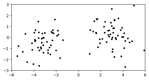
NUMERICAL CORNER: We will apply it to our previous two-cluster example. The necessary functions are in mmids.py, which is available on the GitHub of the book.
seed = 42
rng = np.random.default_rng(seed)
d, n, w = 10, 100, 3.
X = mmids.two_mixed_clusters(rng, d, n, w)
plt.figure(figsize=(6,3))
plt.scatter(X[:,0], X[:,1], s=10, c='k')
plt.axis([-6,6,-3,3])
plt.show()
Let’s compute the top singular vector.
u, s, v = topsing(rng, X)
print(v)
[ 0.99257882  0.10164805  0.01581003  0.03202184  0.02075852  0.02798115
 -0.02920916 -0.028189   -0.0166094  -0.00648726]
This is approximately \(-\mathbf{e}_1\). We get roughly the same answer (possibly up to sign) from Python’s numpy.linalg.svd function.
u, s, vh = LA.svd(X)
print(vh.T[:,0])
[ 0.99257882  0.10164803  0.01581003  0.03202184  0.02075851  0.02798112
 -0.02920917 -0.028189   -0.01660938 -0.00648724]
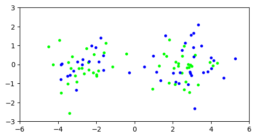
Recall that, when we applied \(k\)-means clustering to this example with \(d=1000\) dimension, we obtained a very poor clustering.
d, n, w = 1000, 100, 3.
X = mmids.two_mixed_clusters(rng, d, n, w)

assign = mmids.kmeans(rng, X, 2)
99423.42794703908
99423.42794703908
99423.42794703908
99423.42794703908
99423.42794703908
plt.figure(figsize=(6,3))
plt.scatter(X[:,0], X[:,1], s=10, c=assign, cmap='brg')
plt.axis([-6,6,-3,3])
plt.show()
Let’s try again, but after projecting on the top singular vector. Recall that this corresponds to finding the best one-dimensional approximating subspace. The projection can be computed using the truncated SVD \(Z= U_{(1)} \Sigma_{(1)} V_{(1)}^T\). We can interpret the rows of \(U_{(1)} \Sigma_{(1)}\) as the coefficients of each data point in the basis \(\mathbf{v}_1\). We will work in that basis. We need one small hack: because our implementation of \(k\)-means clustering expects data points in at least \(2\) dimension, we add a column of \(0\)’s.
u, s, v = topsing(rng, X)
Xproj = np.stack((u*s, np.zeros(np.shape(X)[0])), axis=-1)
fig = plt.figure()
ax = fig.add_subplot(111, aspect='equal')
ax.scatter(Xproj[:,0], Xproj[:,1], s=10, c='b', alpha=0.25)
plt.ylim([-3,3])
plt.show()
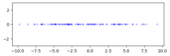
There is a small – yet noticeable – gap around 0. We run \(k\)-means clustering on the projected data.
assign = mmids.kmeans(rng, Xproj, 2)
1779.020119584778
514.1899426112672
514.1899426112672
514.1899426112672
514.1899426112672
Show code cell source
plt.figure(figsize=(6,3))
plt.scatter(X[:,0], X[:,1], s=10, c=assign, cmap='brg')
plt.axis([-6,6,-3,3])
plt.show()
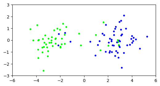
Much better. We give a more formal explanation of this outcome in a subsequent section. In essence, quoting [BHK, Section 7.5.1]:
[…] let’s understand the central advantage of doing the projection to [the top \(k\) right singular vectors]. It is simply that for any reasonable (unknown) clustering of data points, the projection brings data points closer to their cluster centers.
Finally, looking at the top right singular vector (or its first ten entries for lack of space), we see that it does align quite well (but not perfectly) with the first dimension.
print(v[:10])
[-0.55564563 -0.02433674  0.02193487 -0.0333936  -0.00445505 -0.00243003
  0.02576056  0.02523275 -0.00682153  0.02524646]
\(\unlhd\)
CHAT & LEARN There are other methods to compute the SVD. Ask your favorite AI chatbot about randomized algorithms for the SVD. What are their advantages in terms of computational efficiency for large matrices? \(\ddagger\)
Self-assessment quiz (with help from Claude, Gemini, and ChatGPT)
1 In the power iteration lemma for the positive semidefinite case, what happens when the initial vector \(\mathbf{x}\) satisfies \(\langle \mathbf{q}_1, \mathbf{x} \rangle < 0\)?
a) The iteration converges to \(\mathbf{q}_1\).
b) The iteration converges to \(-\mathbf{q}_1\).
c) The iteration does not converge.
d) The iteration converges to a random eigenvector.
2 In the power iteration lemma for the SVD case, what is the convergence result for a random vector \(\mathbf{x}\)?
a) \(B^k \mathbf{x} / \|B^k \mathbf{x}\|\) converges to \(\mathbf{u}_1\).
b) \(B^k \mathbf{x} / \|B^k \mathbf{x}\|\) converges to \(\mathbf{v}_1\) or \(-\mathbf{v}_1\).
c) \(B^k \mathbf{x} / \|B^k \mathbf{x}\|\) converges to \(\sigma_1\).
d) \(B^k \mathbf{x} / \|B^k \mathbf{x}\|\) does not converge.
3 Suppose you apply the power iteration method to a matrix \(A\) and obtain a vector \(\mathbf{v}\). How can you compute the corresponding singular value \(\sigma\) and left singular vector \(\mathbf{u}\)?
a) \(\sigma = \|A\mathbf{v}\|\) and \(\mathbf{u} = A\mathbf{v}/\sigma\)
b) \(\sigma = \|A^T\mathbf{v}\|\) and \(\mathbf{u} = A^T\mathbf{v}/\sigma\)
c) \(\sigma = \|\mathbf{v}\|\) and \(\mathbf{u} = \mathbf{v}/\sigma\)
d) \(\sigma = 1\) and \(\mathbf{u} = A\mathbf{v}\)
4 What is required for the initial vector \(\mathbf{x}\) in the power iteration method to ensure convergence to the top eigenvector?
a) \(\mathbf{x}\) must be a zero vector.
b) \(\mathbf{x}\) must be orthogonal to the top eigenvector.
c) \(\langle \mathbf{q}_1, \mathbf{x} \rangle \neq 0\).
d) \(\mathbf{x}\) must be the top eigenvector itself.
5 What does the truncated SVD \(Z = U_{(2)} \Sigma_{(2)} V_{(2)}^T\) correspond to? [Uses Section 4.8.2.1.]
a) The best one-dimensional approximating subspace
b) The best two-dimensional approximating subspace
c) The projection of the data onto the top singular vector
d) The projection of the data onto the top two singular vectors
Answer for 1: b. Justification: The lemma states that if \(\langle \mathbf{q}_1, \mathbf{x} \rangle < 0\), then the limit of \(A^k \mathbf{x} / \|A^k \mathbf{x}\|\) is \(-\mathbf{q}_1\).
Answer for 2: b. Justification: The lemma states that if \(\langle \mathbf{v}_1, \mathbf{x} \rangle > 0\), then \(B^k \mathbf{x} / \|B^k \mathbf{x}\|\) converges to \(\mathbf{v}_1\), and if \(\langle \mathbf{v}_1, \mathbf{x} \rangle < 0\), then the limit is \(-\mathbf{v}_1\).
Answer for 3: a. Justification: The text provides these formulas in the “Numerical Corner” section.
Answer for 4: c. Justification: The key lemma states that convergence is ensured if \(\mathbf{x}\) is such that \(\langle \mathbf{q}_1, \mathbf{x} \rangle \neq 0\).
Answer for 5: d. Justification: The text states that “projecting on the top two singular vectors… corresponds to finding the best two-dimensional approximating subspace. The projection can be computed using the truncated SVD \(Z = U_{(2)} \Sigma_{(2)} V_{(2)}^T\).”