\(\newcommand{\bmu}{\boldsymbol{\mu}}\) \(\newcommand{\bSigma}{\boldsymbol{\Sigma}}\) \(\newcommand{\bfbeta}{\boldsymbol{\beta}}\) \(\newcommand{\bflambda}{\boldsymbol{\lambda}}\) \(\newcommand{\bgamma}{\boldsymbol{\gamma}}\) \(\newcommand{\bsigma}{{\boldsymbol{\sigma}}}\) \(\newcommand{\bpi}{\boldsymbol{\pi}}\) \(\newcommand{\btheta}{{\boldsymbol{\theta}}}\) \(\newcommand{\bphi}{\boldsymbol{\phi}}\) \(\newcommand{\balpha}{\boldsymbol{\alpha}}\) \(\newcommand{\blambda}{\boldsymbol{\lambda}}\) \(\renewcommand{\P}{\mathbb{P}}\) \(\newcommand{\E}{\mathbb{E}}\) \(\newcommand{\indep}{\perp\!\!\!\perp} \newcommand{\bx}{\mathbf{x}}\) \(\newcommand{\bp}{\mathbf{p}}\) \(\renewcommand{\bx}{\mathbf{x}}\) \(\newcommand{\bX}{\mathbf{X}}\) \(\newcommand{\by}{\mathbf{y}}\) \(\newcommand{\bY}{\mathbf{Y}}\) \(\newcommand{\bz}{\mathbf{z}}\) \(\newcommand{\bZ}{\mathbf{Z}}\) \(\newcommand{\bw}{\mathbf{w}}\) \(\newcommand{\bW}{\mathbf{W}}\) \(\newcommand{\bv}{\mathbf{v}}\) \(\newcommand{\bV}{\mathbf{V}}\) \(\newcommand{\bfg}{\mathbf{g}}\) \(\newcommand{\bfh}{\mathbf{h}}\) \(\newcommand{\horz}{\rule[.5ex]{2.5ex}{0.5pt}}\) \(\renewcommand{\S}{\mathcal{S}}\) \(\newcommand{\X}{\mathcal{X}}\) \(\newcommand{\var}{\mathrm{Var}}\) \(\newcommand{\pa}{\mathrm{pa}}\) \(\newcommand{\Z}{\mathcal{Z}}\) \(\newcommand{\bh}{\mathbf{h}}\) \(\newcommand{\bb}{\mathbf{b}}\) \(\newcommand{\bc}{\mathbf{c}}\) \(\newcommand{\cE}{\mathcal{E}}\) \(\newcommand{\cP}{\mathcal{P}}\) \(\newcommand{\bbeta}{\boldsymbol{\beta}}\) \(\newcommand{\bLambda}{\boldsymbol{\Lambda}}\) \(\newcommand{\cov}{\mathrm{Cov}}\) \(\newcommand{\bfk}{\mathbf{k}}\) \(\newcommand{\idx}[1]{}\) \(\newcommand{\xdi}{}\)

4.6. Further applications of the SVD: low-rank approximations and ridge regression

In this section, we discuss further properties of the SVD. We first introduce additional matrix norms.

4.6.1. Matrix norms

Recall that the Frobenius norm\(\idx{Frobenius norm}\xdi\) of an \(n \times m\) matrix \(A = (a_{i,j})_{i,j} \in \mathbb{R}^{n \times m}\) is defined as

\[ \|A\|_F = \sqrt{\sum_{i=1}^n \sum_{j=1}^m a_{i,j}^2}. \]

Here we introduce a different notion of matrix norm that has many uses in data science (and beyond).

Induced norm The Frobenius norm does not directly relate to \(A\) as a representation of a linear map. In particular, it is desirable in many contexts to quantify how two matrices differ in terms of how they act on vectors. For instance, one is often interested in bounding quantities of the following form. Let \(B, B' \in \mathbb{R}^{n \times m}\) and let \(\mathbf{x} \in \mathbb{R}^m\) be of unit norm. What can be said about \(\|B \mathbf{x} - B' \mathbf{x}\|\)? Intuitively, what we would like is this: if the norm of \(B - B'\) is small then \(B\) is close to \(B'\) as a linear map, that is, the vector norm \(\|B \mathbf{x} - B' \mathbf{x}\|\) is small for any unit vector \(\mathbf{x}\). The following definition provides us with such a notion. Define the unit sphere \(\mathbb{S}^{m-1} = \{\mathbf{x} \in \mathbb{R}^m\,:\,\|\mathbf{x}\| = 1\}\) in \(m\) dimensions.

DEFINITION (\(2\)-Norm) The \(2\)-norm of a matrix\(\idx{2-norm}\xdi\) \(A \in \mathbb{R}^{n \times m}\) is

\[ \|A\|_2 = \max_{\mathbf{0} \neq \mathbf{x} \in \mathbb{R}^m} \frac{\|A \mathbf{x}\|}{\|\mathbf{x}\|} = \max_{\mathbf{x} \in \mathbb{S}^{m-1}} \|A \mathbf{x}\|. \]

\(\natural\)

The equality in the definition uses the absolute homogeneity of the vector norm. Also the definition implicitly uses the Extreme Value Theorem. In this case, we use the fact that the function \(f(\mathbf{x}) = \|A \mathbf{x}\|\) is continuous and the set \(\mathbb{S}^{m-1}\) is closed and bounded to conclude that there exists \(\mathbf{x}^* \in \mathbb{S}^{m-1}\) such that \(f(\mathbf{x}^*) \geq f(\mathbf{x})\) for all \(\mathbf{x} \in \mathbb{S}^{m-1}\).

The \(2\)-norm of a matrix has many other useful properties. The first four below are what makes it a norm.

LEMMA (Properties of the \(2\)-Norm) Let \(A, B \in \mathbb{R}^{n \times m}\) and \(\alpha \in \mathbb{R}\). The following hold:

a) \(\|A\|_2 \geq 0\)

b) \(\|A\|_2 = 0\) if and only if \(A = 0\)

c) \(\|\alpha A\|_2 = |\alpha| \|A\|_2\)

d) \(\|A + B \|_2 \leq \|A\|_2 + \|B\|_2\)

e) \(\|A B \|_2 \leq \|A\|_2 \|B\|_2\).

f) \(\|A \mathbf{x}\| \leq \|A\|_2 \|\mathbf{x}\|\), \(\forall \mathbf{0} \neq \mathbf{x} \in \mathbb{R}^m\)

\(\flat\)

Proof: These properties all follow from the definition of the \(2\)-norm and the corresponding properties for the vector norm:

• Claims a) and f) are immediate from the definition.

• For b) note that \(\|A\|_2 = 0\) implies \(\|A \mathbf{x}\|_2 = 0, \forall \mathbf{x} \in \mathbb{S}^{m-1}\), so that \(A \mathbf{x} = \mathbf{0}, \forall \mathbf{x} \in \mathbb{S}^{m-1}\). In particular, \(a_{ij} = \mathbf{e}_i^T A \mathbf{e}_j = 0, \forall i,j\).

• For c), d), e), observe that for all \(\mathbf{x} \in \mathbb{S}^{m-1}\)

\[ \|\alpha A \mathbf{x}\| = |\alpha| \|A \mathbf{x}\|, \]

\[\|(A+B)\mathbf{x}\| = \|A\mathbf{x} + B\mathbf{x}\| \leq \|A\mathbf{x}\| + \|B\mathbf{x}\| \leq \|A\|_2 + \|B\|_2 \]

\[ \|(AB)\mathbf{x}\| = \|A(B\mathbf{x})\| \leq \|A\|_2 \|B\mathbf{x}\| \leq \|A\|_2 \|B\|_2.\]

Then apply the definition of \(2\)-norm. For example, for ©,

\[\begin{align*} \|\alpha A\|_2 &= \max_{\mathbf{x} \in \mathbb{S}^{m-1}} \|\alpha A \mathbf{x}\|\\ &= \max_{\mathbf{x} \in \mathbb{S}^{m-1}} |\alpha| \|A \mathbf{x}\|\\ &= |\alpha| \max_{\mathbf{x} \in \mathbb{S}^{m-1}} \|A \mathbf{x}\|\\ &= |\alpha| \|A\|_2, \end{align*}\]

where we used that \(|\alpha|\) does not depend on \(\mathbf{x}\). \(\square\)

NUMERICAL CORNER: In Numpy, the Frobenius norm of a matrix can be computed using the default of the function numpy.linalg.norm while the induced norm can be computed using the same function with ord parameter set to 2.

A = np.array([[1., 0.],[0., 1.],[0., 0.]])
print(A)

[[1. 0.]
 [0. 1.]
 [0. 0.]]

LA.norm(A)

1.4142135623730951

LA.norm(A, 2)

1.0

\(\unlhd\)

Matrix norms and SVD As it turns out, the two notions of matrix norms we have introduced admit simple expressions in terms of the singular values of the matrix.

LEMMA (Matrix Norms and Singular Values) \(\idx{matrix norms and singular values lemma}\xdi\) Let \(A \in \mathbb{R}^{n \times m}\) be a matrix with compact SVD

\[ A = \sum_{\ell=1}^r \sigma_\ell \mathbf{u}_\ell \mathbf{v}_\ell^T \]

where recall that \(\sigma_1 \geq \sigma_2 \geq \cdots \sigma_r > 0\). Then

\[ \|A\|^2_F = \sum_{\ell=1}^r \sigma_\ell^2 \]

and

\[ \|A\|^2_2 = \sigma_{1}^2. \]

\(\flat\)

Proof: We will use the notation \(\mathbf{v}_\ell = (v_{\ell,1},\ldots,v_{\ell,m})^T\). Using that the squared Frobenius norm of \(A\) is the sum of the squared norms of its columns, we have

\[ \|A\|^2_F = \left\|\sum_{\ell=1}^r \sigma_\ell \mathbf{u}_\ell \mathbf{v}_\ell^T\right\|_F^2 = \sum_{j=1}^m \left\|\sum_{\ell=1}^r \sigma_\ell v_{\ell,j} \mathbf{u}_\ell \right\|^2. \]

Because the \(\mathbf{u}_\ell\)’s are orthonormal, this is

\[ \sum_{j=1}^m \sum_{\ell=1}^r \sigma_\ell^2 v_{\ell,j}^2 = \sum_{\ell=1}^r \sigma_\ell^2 \left(\sum_{j=1}^m v_{\ell,j}^2\right) = \sum_{\ell=1}^r \sigma_\ell^2 \|\mathbf{v}_{\ell}\|^2 = \sum_{\ell=1}^r \sigma_\ell^2, \]

where we used that the \(\mathbf{v}_\ell\)’s are also orthonormal.

For the second claim, recall that the \(2\)-norm is defined as

\[ \|A\|_2^2 = \max_{\mathbf{x} \in \mathbb{S}^{m-1}} \|A \mathbf{x}\|^2. \]

We have shown previously that \(\mathbf{v}_1\) solves this problem. Hence \(\|A\|_2^2 = \|A \mathbf{v}_1\|^2 = \sigma_1^2\). \(\square\)

4.6.2. Low-rank approximation

Now that we have defined a notion of distance between matrices, we will consider the problem of finding a good approximation to a matrix \(A\) among all matrices of rank at most \(k\). We will start with the Frobenius norm, which is easier to work with, and we will show later on that the solution is the same under the induced norm. The solution to this problem will be familiar. In essence, we will re-interpret our solution to the best approximating subspace as a low-rank approximation.

Low-rank approximation in the Frobenius norm \(\idx{low-rank approximation}\xdi\) From the proof of the Row Rank Equals Column Rank Lemma, it follows that a rank-\(r\) matrix \(A\) can be written as a sum of \(r\) rank-\(1\) matrices

\[ A = \sum_{i=1}^r \mathbf{b}_i \mathbf{c}_i^T. \]

We will now consider the problem of finding a “simpler” approximation to \(A\)

\[ A \approx \sum_{i=1}^k \mathbf{b}'_i (\mathbf{c}'_i)^T \]

where \(k < r\). Here we measure the quality of this approximation using a matrix norm.

We are ready to state our key observation. In words, the best rank-\(k\) approximation to \(A\) in Frobenius norm is obtained by projecting the rows of \(A\) onto a linear subspace of dimension \(k\). We will come back to how one finds the best such subspace below. (Hint: We have already solved this problem.)

LEMMA (Projection and Rank-\(k\) Approximation) \(\idx{projection and rank-k approximation lemma}\xdi\) Let \(A \in \mathbb{R}^{n \times m}\). For any matrix \(B \in \mathbb{R}^{n \times m}\) of rank \(k \leq \min\{n,m\}\),

\[ \|A - B_{\perp}\|_F \leq \|A - B\|_F \]

where \(B_{\perp} \in \mathbb{R}^{n \times m}\) is the matrix of rank at most \(k\) obtained as follows. Denote row \(i\) of \(A\), \(B\) and \(B_{\perp}\) respectively by \(\boldsymbol{\alpha}_i^T\), \(\mathbf{b}_{i}^T\) and \(\mathbf{b}_{\perp,i}^T\), \(i=1,\ldots, n\). Set \(\mathbf{b}_{\perp,i}\) to be the orthogonal projection of \(\boldsymbol{\alpha}_i\) onto \(\mathcal{Z} = \mathrm{span}(\mathbf{b}_1,\ldots,\mathbf{b}_n)\). \(\flat\)

Proof idea: The square of the Frobenius norm decomposes as a sum of squared row norms. Each term in the sum is minimized by the orthogonal projection.

Proof: By definition of the Frobenius norm, we note that

\[ \|A - B\|_F^2 = \sum_{i=1}^n \sum_{j=1}^m (a_{i,j} - b_{i,j})^2 = \sum_{i=1}^n \|\boldsymbol{\alpha}_i - \mathbf{b}_{i}\|^2 \]

and similarly for \(\|A - B_{\perp}\|_F\). We make two observations:

1. Because the orthogonal projection of \(\boldsymbol{\alpha}_i\) onto \(\mathcal{Z}\) minimizes the distance to \(\mathcal{Z}\), it follows that term by term \(\|\boldsymbol{\alpha}_i - \mathbf{b}_{\perp,i}\| \leq \|\boldsymbol{\alpha}_i - \mathbf{b}_{i}\|\) so that

\[ \|A - B_\perp\|_F^2 = \sum_{i=1}^n \|\boldsymbol{\alpha}_i - \mathbf{b}_{\perp,i}\|^2 \leq \sum_{i=1}^n \|\boldsymbol{\alpha}_i - \mathbf{b}_{i}\|^2 = \|A - B\|_F^2. \]

2. Moreover, because the projections satisfy \(\mathbf{b}_{\perp,i} \in \mathcal{Z}\) for all \(i\), \(\mathrm{row}(B_\perp) \subseteq \mathrm{row}(B)\) and, hence, the rank of \(B_\perp\) is at most the rank of \(B\).

That concludes the proof. \(\square\)

Recall the approximating subspace problem. That is, think of the rows \(\boldsymbol{\alpha}_i^T\) of \(A \in \mathbb{R}^{n \times m}\) as a collection of \(n\) data points in \(\mathbb{R}^m\). We are looking for a linear subspace \(\mathcal{Z}\) that minimizes \(\sum_{i=1}^n \|\boldsymbol{\alpha}_i - \mathrm{proj}_\mathcal{Z}(\boldsymbol{\alpha}_i)\|^2\) over all linear subspaces of \(\mathbb{R}^m\) of dimension at most \(k\). By the Projection and Rank-\(k\) Approximation Lemma, this problem is equivalent to finding a matrix \(B\) that minimizes \(\|A - B\|_F\) among all matrices in \(\mathbb{R}^{n \times m}\) of rank at most \(k\). Of course we have solved this problem before.

Let \(A \in \mathbb{R}^{n \times m}\) be a matrix with SVD \(A = \sum_{j=1}^r \sigma_j \mathbf{u}_j \mathbf{v}_j^T\). For \(k < r\), truncate the sum at the \(k\)-th term \(A_k = \sum_{j=1}^k \sigma_j \mathbf{u}_j \mathbf{v}_j^T\). The rank of \(A_k\) is exactly \(k\). Indeed, by construction,

1. the vectors \(\{\mathbf{u}_j\,:\,j = 1,\ldots,k\}\) are orthonormal, and

2. since \(\sigma_j > 0\) for \(j=1,\ldots,k\) and the vectors \(\{\mathbf{v}_j\,:\,j = 1,\ldots,k\}\) are orthonormal, \(\{\mathbf{u}_j\,:\,j = 1,\ldots,k\}\) spans the column space of \(A_k\).

We have shown before that \(A_k\) is the best approximation to \(A\) among matrices of rank at most \(k\) in Frobenius norm. Specifically, the Greedy Finds Best Fit Theorem implies that, for any matrix \(B \in \mathbb{R}^{n \times m}\) of rank at most \(k\),

\[ \|A - A_k\|_F \leq \|A - B\|_F. \]

This result is known as the Eckart-Young Theorem\(\idx{Eckart-Young theorem}\xdi\). It also holds in the induced \(2\)-norm, as we show next.

Low-rank approximation in the induced norm We show in this section that the same holds in the induced norm. First, some observations.

LEMMA (Matrix Norms and Singular Values: Truncation) Let \(A \in \mathbb{R}^{n \times m}\) be a matrix with SVD

\[ A = \sum_{j=1}^r \sigma_j \mathbf{u}_j \mathbf{v}_j^T \]

where recall that \(\sigma_1 \geq \sigma_2 \geq \cdots \sigma_r > 0\) and let \(A_k\) be the truncation defined above. Then

\[ \|A - A_k\|^2_F = \sum_{j=k+1}^r \sigma_j^2 \]

and

\[ \|A - A_k\|^2_2 = \sigma_{k+1}^2. \]

\(\flat\)

Proof: For the first claim, by definition, summing over the columns of \(A - A_k\)

\[ \|A - A_k\|^2_F = \left\|\sum_{j=k+1}^r \sigma_j \mathbf{u}_j \mathbf{v}_j^T\right\|_F^2 = \sum_{i=1}^m \left\|\sum_{j=k+1}^r \sigma_j v_{j,i} \mathbf{u}_j \right\|^2. \]

Because the \(\mathbf{u}_j\)’s are orthonormal, this is

\[ \sum_{i=1}^m \sum_{j=k+1}^r \sigma_j^2 v_{j,i}^2 = \sum_{j=k+1}^r \sigma_j^2 \left(\sum_{i=1}^m v_{j,i}^2\right) = \sum_{j=k+1}^r \sigma_j^2 \]

where we used that the \(\mathbf{v}_j\)’s are also orthonormal.

For the second claim, recall that the induced norm is defined as

\[ \|B\|_2 = \max_{\mathbf{x} \in \mathbb{S}^{m-1}} \|B \mathbf{x}\|. \]

For any \(\mathbf{x} \in \mathbb{S}^{m-1}\)

\[ \left\|(A - A_k)\mathbf{x}\right\|^2 = \left\| \sum_{j=k+1}^r \sigma_j \mathbf{u}_j (\mathbf{v}_j^T \mathbf{x}) \right\|^2 = \sum_{j=k+1}^r \sigma_j^2 \langle \mathbf{v}_j, \mathbf{x}\rangle^2. \]

Because the \(\sigma_j\)’s are in decreasing order, this is maximized when \(\langle \mathbf{v}_j, \mathbf{x}\rangle = 1\) if \(j=k+1\) and \(0\) otherwise. That is, we take \(\mathbf{x} = \mathbf{v}_{k+1}\) and the norm is then \(\sigma_{k+1}^2\), as claimed. \(\square\)

THEOREM (Low-Rank Approximation in the Induced Norm) \(\idx{low-rank approximation in the induced norm theorem}\xdi\) Let \(A \in \mathbb{R}^{n \times m}\) be a matrix with SVD

\[ A = \sum_{j=1}^r \sigma_j \mathbf{u}_j \mathbf{v}_j^T \]

and let \(A_k\) be the truncation defined above with \(k < r\). For any matrix \(B \in \mathbb{R}^{n \times m}\) of rank at most \(k\),

\[ \|A - A_k\|_2 \leq \|A - B\|_2. \]

\(\sharp\)

Proof idea: We know that \(\|A - A_k\|_2^2 = \sigma_{k+1}^2\). So we want to lower bound \(\|A - B\|_2^2\) by \(\sigma_{k+1}^2\). For that, we have to find an appropriate \(\mathbf{z}\) for any given \(B\) of rank at most \(k\). The idea is to take a vector \(\mathbf{z}\) in the intersection of the null space of \(B\) and the span of the singular vectors \(\mathbf{v}_1,\ldots,\mathbf{v}_{k+1}\). By the former, the squared norm of \((A - B)\mathbf{z}\) is equal to the squared norm of \(A\mathbf{z}\) which lower bounds \(\|A\|_2^2\). By the latter, \(\|A \mathbf{z}\|^2\) is at least \(\sigma_{k+1}^2\).

Proof: By the Rank-Nullity Theorem, the dimension of \(\mathrm{null}(B)\) is at least \(m-k\) so there is a unit vector \(\mathbf{z}\) in the intersection

\[ \mathbf{z} \in \mathrm{null}(B) \cap \mathrm{span}(\mathbf{v}_1,\ldots,\mathbf{v}_{k+1}). \]

(Prove it!) Then \((A-B)\mathbf{z} = A\mathbf{z}\) since \(\mathbf{z} \in \mathrm{null}(B)\). Also since \(\mathbf{z} \in \mathrm{span}(\mathbf{v}_1,\ldots,\mathbf{v}_{k+1})\), and therefore orthogonal to \(\mathbf{v}_{k+2},\ldots,\mathbf{v}_r\), we have

\[\begin{align*} \|(A-B)\mathbf{z}\|^2 &= \|A\mathbf{z}\|^2\\ &= \left\|\sum_{j=1}^r \sigma_j \mathbf{u}_j \mathbf{v}_j^T\mathbf{z}\right\|^2\\ &= \left\|\sum_{j=1}^{k+1} \sigma_j \mathbf{u}_j \mathbf{v}_j^T\mathbf{z}\right\|^2\\ &= \sum_{j=1}^{k+1} \sigma_j^2 \langle \mathbf{v}_j, \mathbf{z}\rangle^2\\ &\geq \sigma_{k+1}^2 \sum_{j=1}^{k+1} \langle \mathbf{v}_j, \mathbf{z}\rangle^2\\ &= \sigma_{k+1}^2. \end{align*}\]

By the Matrix Norms and Singular Values Lemma, \(\sigma_{k+1}^2 = \|A - A_k\|_2\) and we are done. \(\square\)

An application: Why project? We return to \(k\)-means clustering and why projecting to a lower-dimensional subspace can produce better results. We prove a simple inequality that provides some insight. Quoting [BHK, Section 7.5.1]:

[…] let’s understand the central advantage of doing the projection to [the top \(k\) right singular vectors]. It is simply that for any reasonable (unknown) clustering of data points, the projection brings data points closer to their cluster centers.

To elaborate, suppose we have \(n\) data points in \(d\) dimensions in the form of the rows \(\mathbf{a}_i^T\), \(i=1\ldots, n\), of matrix \(A \in \mathbb{A}^{n \times d}\), where we assume that \(n > d\) and that \(A\) has full column rank. Imagine these data points come from an unknown ground-truth \(k\)-clustering assignment \(g(i) \in [k]\), \(i = 1,\ldots, n\), with corresponding unknown centers \(\mathbf{c}_j\), \(j = 1,\ldots, k\), for \(g(i) = j\). Let \(C \in \mathbb{R}^{n \times d}\) be the corresponding matrix, that is, row \(i\) of \(C\) is \(\mathbf{c}_j^T\) if \(g(i) = j\). The \(k\)-means objective of the true clustering is then

(4.1)\[\begin{align} \sum_{j\in [k]} \sum_{i:g(i)=j} \|\mathbf{a}_i - \mathbf{c}_{j}\|^2 &= \sum_{j\in [k]} \sum_{i:g(i)=j} \sum_{\ell=1}^d (a_{i,\ell} - c_{j,\ell})^2\\ &= \sum_{i=1}^n \sum_{\ell=1}^d (a_{i,\ell} - c_{g(i),\ell})^2\\ &= \|A - C\|_F^2. \end{align}\]

The matrix \(A\) has an SVD \(A = \sum_{j=1}^r \sigma_j \mathbf{u}_j \mathbf{v}_j^T\) and for \(k < r\) we have the truncation \(A_k = \sum_{j=1}^k \sigma_j \mathbf{u}_j \mathbf{v}_j^T\). It corresponds to projecting each row of \(A\) onto the linear subspace spanned by the first \(k\) right singular vectors \(\mathbf{v}_1, \ldots, \mathbf{v}_k\). To see this, note that the \(i\)-th row of \(A\) is \(\boldsymbol{\alpha}_i^T = \sum_{j=1}^r \sigma_j u_{j,i} \mathbf{v}_j^T\) and that, because the \(\mathbf{v}_j\)’s are linearly independent and in particular \(\mathbf{v}_1,\ldots,\mathbf{v}_k\) is an orthonormal basis of its span, the projection of \(\boldsymbol{\alpha}_i\) onto \(\mathrm{span}(\mathbf{v}_1,\ldots,\mathbf{v}_k)\) is

\[ \sum_{\ell=1}^k \mathbf{v}_\ell \left\langle\sum_{j=1}^r \sigma_j u_{j,i} \mathbf{v}_j,\mathbf{v}_\ell\right\rangle = \sum_{\ell=1}^k \sigma_\ell u_{\ell,i} \mathbf{v}_\ell \]

which is the \(i\)-th row of \(A_k\). The \(k\)-means objective of \(A_k\) with respect to the ground-truth centers \(\mathbf{c}_j\), \(j=1,\ldots,k\), is \(\|A_k - C\|_F^2\).

One more observation: the rank of \(C\) is at most \(k\). Indeed, there are \(k\) different rows in \(C\) so its row rank is \(k\) if these different rows are linearly independent and less than \(k\) otherwise.

THEOREM (Why Project) \(\idx{why project theorem}\xdi\) Let \(A \in \mathbb{A}^{n \times d}\) be a matrix and let \(A_k\) be the truncation above. For any matrix \(C \in \mathbb{R}^{n \times d}\) of rank \(\leq k\),

\[ \|A_k - C\|_F^2 \leq 8 k \|A - C\|_2^2. \]

\(\sharp\)

The content of this inequality is the following. The quantity \(\|A_k - C\|_F^2\) is the \(k\)-means objective of the projection \(A_k\) with respect to the true centers, that is, the sum of the squared distances to the centers. By the Matrix Norms and Singular Values Lemma, the inequality above gives that

\[ \|A_k - C\|_F^2 \leq 8 k \sigma_1(A - C)^2, \]

where \(\sigma_j(A - C)\) is the \(j\)-th singular value of \(A - C\). On the other hand, by the same lemma, the \(k\)-means objective of the un-projected data is

\[ \|A - C\|_F^2 = \sum_{j=1}^{\mathrm{rk}(A-C)} \sigma_j(A - C)^2. \]

If the rank of \(A-C\) is much larger than \(k\) and the singular values of \(A-C\) decay slowly, then the latter quantity may be much larger. In other words, projecting may bring the data points closer to their true centers, potentially making it easier to cluster them.

Proof: (Why Project) We have shown previously that, for any matrices \(A, B \in \mathbb{R}^{n \times m}\), the rank of their sum is less or equal than the sum of their ranks, that is, \(\mathrm{rk}(A+B) \leq \mathrm{rk}(A) + \mathrm{rk}(B)\). So the rank of the difference \(A_k - C\) is at most the sum of the ranks

\[ \mathrm{rk}(A_k - C) \leq \mathrm{rk}(A_k) + \mathrm{rk}(-C) \leq 2 k \]

where we used that the rank of \(A_k\) is \(k\) and the rank of \(C\) is \(\leq k\) since it has \(k\) distinct rows. By the Matrix Norms and Singular Values Lemma,

\[ \|A_k - C\|_F^2 \leq 2k \|A_k - C\|_2^2. \]

By the triangle inequality for matrix norms,

\[ \|A_k - C\|_2 \leq \|A_k - A\|_2 + \|A - C\|_2. \]

By the Low-Rank Approximation in the Induced Norm Theorem,

\[ \|A - A_k\|_2 \leq \|A - C\|_2 \]

since \(C\) has rank at most \(k\). Putting these three inequalities together,

\[ \|A_k - C\|_F^2 \leq 2k (2 \|A - C\|_2)^2 = 8k \|A - C\|_2^2. \]

\(\square\)

NUMERICAL CORNER: We return to our example with the two Gaussian clusters. We use function producing two separate clusters.

def two_separate_clusters(rng, d, n, w):
    
    mu0 = np.concatenate(([w], np.zeros(d-1)))
    mu1 = np.concatenate(([-w], np.zeros(d-1)))
    
    X0 = mmids.spherical_gaussian(rng, d, n, mu0, 1)
    X1 = mmids.spherical_gaussian(rng, d, n, mu1, 1)
    
    return X0, X1

We first generate the data.

seed = 535
rng = np.random.default_rng(seed)
d, n, w = 1000, 100, 3.
X1, X2 = two_separate_clusters(rng, d, n, w)
X = np.vstack((X1, X2))

In reality, we cannot compute the matrix norms of \(X-C\) and \(X_k-C\) as the true centers are not known. But, because this is simulated data, we happen to know the truth and we can check the validity of our results in this case. The centers are:

C1 = np.stack([np.concatenate(([-w], np.zeros(d-1))) for _ in range(n)])
C2 = np.stack([np.concatenate(([w], np.zeros(d-1))) for _ in range(n)])
C = np.vstack((C1, C2))

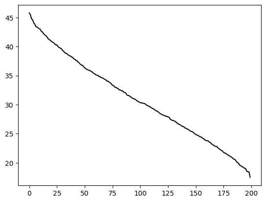
We use numpy.linalg.svd function to compute the norms from the formulas in the Matrix Norms and Singular Values Lemma. First, we observe that the singular values of \(X-C\) are decaying slowly.

uc, sc, vhc = LA.svd(X-C)
plt.plot(sc, c='k')
plt.show()

The \(k\)-means objective with respect to the true centers under the full-dimensional data is:

print(np.sum(sc**2))

207905.47916782406

while the square of the top singular value of \(X-C\) is only:

print(sc[0]**2)

8258.19604762502

Finally, we compute the \(k\)-means objective with respect to the true centers under the projected one-dimensional data:

u, s, vh = LA.svd(X)
print(np.sum((s[0] * np.outer(u[:,0],vh[:,0]) - C)**2))

8099.057045408984

\(\unlhd\)

CHAT & LEARN Ask your AI chatbot about the applications of SVD in recommendation systems. How is it used to predict user preferences? \(\ddagger\)

CHAT & LEARN Ask your favorite AI chatbot about nonnegative matrix factorization (NMF) and how it compares to SVD. What are the key differences in their constraints and applications? How does NMF handle interpretability in topics like text analysis or image processing? Explore some algorithms used to compute NMF. \(\ddagger\)

4.6.3. Ridge regression

Here we consider what is called Tikhonov regularization\(\idx{Tikhonov regularization}\xdi\), an idea that idea turns out to be useful in overdetermined linear systems, particularly when the columns of the matrix \(A\) are linearly dependent or close to linearly dependent (which is sometimes referred as multicollinearity\(\idx{multicollinearity}\xdi\) in statistics). It trades off minimizing the fit to the data versus minimizing the norm of the solution. More precisely, for a parameter \(\lambda > 0\) to be chosen, we solve\(\idx{ridge regression}\xdi\)

\[ \min_{\mathbf{x} \in \mathbb{R}^m} \|A \mathbf{x} - \mathbf{b}\|_2^2 + \lambda \|\mathbf{x}\|_2^2. \]

The second term is referred to as an \(L_2\)-regularizer\(\idx{L2-regularization}\xdi\). Here \(A \in \mathbb{R}^{n\times m}\) with \(n \geq m\) and \(\mathbf{b} \in \mathbb{R}^n\).

To solve this optimization problem, we show that the objective function is strongly convex. We then find its unique stationary point. Rewriting the objective in quadratic function form

\[\begin{align*} f(\mathbf{x}) &= \|A \mathbf{x} - \mathbf{b}\|_2^2 + \lambda \|\mathbf{x}\|_2^2\\ &= \mathbf{x}^T A^T A \mathbf{x} - 2 \mathbf{b}^T A \mathbf{x} + \mathbf{b}^T \mathbf{b} + \lambda \mathbf{x}^T \mathbf{x}\\ &= \mathbf{x}^T (A^T A + \lambda I_{m \times m}) \mathbf{x} - 2 \mathbf{b}^T A \mathbf{x} + \mathbf{b}^T \mathbf{b}\\ &= \frac{1}{2} \mathbf{x}^T P \mathbf{x} + \mathbf{q}^T \mathbf{x} + r, \end{align*}\]

where \(P = 2 (A^T A + \lambda I_{m \times m})\) is symmetric, \(\mathbf{q} = - 2 A^T \mathbf{b}\), and \(r= \mathbf{b}^T \mathbf{b} = \|\mathbf{b}\|^2\).

As we previously computed, the Hessian of \(f\) is \(H_f(\mathbf{x})= P\). Now comes a key observation. The matrix \(P\) is positive definite whenever \(\lambda > 0\). Indeed, for any \(\mathbf{z} \in \mathbb{R}^m\),

\[ \mathbf{z}^T [2 (A^T A + \lambda I_{m \times m})] \mathbf{z} = 2 \|A \mathbf{z}\|_2^2 + 2 \lambda \|\mathbf{z}\|_2^2 > 0. \]

Let \(\mu = 2 \lambda > 0\). Then \(f\) is \(\mu\)-strongly convex. This holds whether or not the columns of \(A\) are linearly independent.

The stationary points are easily characterized. Recall that the gradient is \(\nabla f(\mathbf{x}) = P \mathbf{x} + \mathbf{q}\). Equating to \(\mathbf{0}\) leads to the system

\[ 2 (A^T A + \lambda I_{m \times m}) \mathbf{x} - 2 A^T \mathbf{b} = \mathbf{0}, \]

that is

\[ \mathbf{x}^{**} = (A^T A + \lambda I_{m \times m})^{-1} A^T \mathbf{b}. \]

The matrix in parenthesis is invertible as it is \(1/2\) of the Hessian, which is positive definite.

Connection to SVD Expressing the solution in terms of a compact SVD \(A = U \Sigma V^T = \sum_{j=1}^r \sigma_j \mathbf{u}_j \mathbf{v}_j^T\) provides some insights into how ridge regression works. Suppose that \(A\) has full column rank. That implies that \(V V^T = I_{m \times m}\). Then observe that

\[\begin{align*} (A^T A + \lambda I_{m \times m})^{-1} &= (V \Sigma U^T U \Sigma V^T + \lambda I_{m \times m})^{-1}\\ &= (V \Sigma^2 V^T + \lambda I_{m \times m})^{-1}\\ &= (V \Sigma^2 V^T + V \lambda I_{m \times m} V^T)^{-1}\\ &= (V [\Sigma^2 + \lambda I_{m \times m}] V^T)^{-1}\\ &= V (\Sigma^2 + \lambda I_{m \times m})^{-1} V^T. \end{align*}\]

Hence

\[ \mathbf{x}^{**} = (A^T A + \lambda I_{m \times m})^{-1} A^T \mathbf{b} = V (\Sigma^2 + \lambda I_{m \times m})^{-1} V^T V \Sigma U^T \mathbf{b} = V (\Sigma^2 + \lambda I_{m \times m})^{-1} \Sigma U^T \mathbf{b}. \]

Our predictions are

\[\begin{align*} A \mathbf{x}^{**} &= U \Sigma V^T V (\Sigma^2 + \lambda I_{m \times m})^{-1} \Sigma U^T \mathbf{b}\\ &= U \Sigma (\Sigma^2 + \lambda I_{m \times m})^{-1} \Sigma U^T \mathbf{b}\\ &= \sum_{j=1}^r \mathbf{u}_j \left\{\frac{\sigma_j^2}{\sigma_j^2 + \lambda} \right\} \mathbf{u}_j^T \mathbf{b}. \end{align*}\]

Note that the terms in curly brackets are \(< 1\) when \(\lambda > 0\).

Compare this to the unregularized least squares solution, which is obtained simply by setting \(\lambda = 0\) above,

\[\begin{align*} A \mathbf{x}^* &= \sum_{j=1}^r \mathbf{u}_j \mathbf{u}_j^T \mathbf{b}. \end{align*}\]

The difference is that the regularized solution reduces the contributions from the left singular vectors corresponding to small singular values.

Self-assessment quiz (with help from Claude, Gemini, and ChatGPT)

1 Which of the following best describes the Frobenius norm of a matrix \(A \in \mathbb{R}^{n \times m}\)?

a) The maximum singular value of \(A\).

b) The square root of the sum of the squares of all entries in \(A\).

c) The maximum absolute row sum of \(A\).

d) The maximum absolute column sum of \(A\).

2 Let \(A \in \mathbb{R}^{n \times m}\) be a matrix with SVD \(A = \sum_{j=1}^r \sigma_j \mathbf{u}_j \mathbf{v}_j^T\) and let \(A_k = \sum_{j=1}^k \sigma_j \mathbf{u}_j \mathbf{v}_j^T\) be the truncated SVD with \(k < r\). Which of the following is true about the Frobenius norm of \(A - A_k\)?

a) \(\|A - A_k\|_F^2 = \sum_{j=1}^k \sigma_j^2\)

b) \(\|A - A_k\|_F^2 = \sum_{j=k+1}^r \sigma_j^2\)

c) \(\|A - A_k\|_F^2 = \sigma_k^2\)

d) \(\|A - A_k\|_F^2 = \sigma_{k+1}^2\)

3 The ridge regression problem is formulated as \(\min_{x \in \mathbb{R}^m} \|Ax - b\|_2^2 + \lambda \|x\|_2^2\). What is the role of the parameter \(\lambda\)?

a) It controls the trade-off between fitting the data and minimizing the norm of the solution.

b) It determines the rank of the matrix \(A\).

c) It is the smallest singular value of \(A\).

d) It is the largest singular value of \(A\).

4 Let \(A\) be an \(n \times m\) matrix with compact SVD \(A = \sum_{j=1}^r \sigma_j u_j v_j^T\). How does the ridge regression solution \(x^{**}\) compare to the least squares solution \(x^*\)?

a) \(x^{**}\) has larger components along the left singular vectors corresponding to small singular values.

b) \(x^{**}\) has smaller components along the left singular vectors corresponding to small singular values.

c) \(x^{**}\) is identical to \(x^*\).

d) None of the above.

5 Let \(A \in \mathbb{R}^{n \times n}\) be a square nonsingular matrix with compact SVD \(A = \sum_{j=1}^n \sigma_j \mathbf{u}_j \mathbf{v}_j^T\). Which of the following is true about the induced 2-norm of the inverse \(A^{-1}\)?

a) \(\|A^{-1}\|_2 = \sigma_1\)

b) \(\|A^{-1}\|_2 = \sigma_n\)

c) \(\|A^{-1}\|_2 = \sigma_1^{-1}\)

d) \(\|A^{-1}\|_2 = \sigma_n^{-1}\)

Answer for 1: b. Justification: The text defines the Frobenius norm of an \(n \times m\) matrix \(A\) as \(\|A\|_F = \sqrt{\sum_{i=1}^{n} \sum_{j=1}^{m} a_{ij}^2}\).

Answer for 2: b. Justification: The text proves that \(\|A - A_k\|_F^2 = \sum_{j=k+1}^r \sigma_j^2\) in the Matrix Norms and Singular Values: Truncation Lemma.

Answer for 3: a. Justification: The text explains that ridge regression “trades off minimizing the fit to the data versus minimizing the norm of the solution,” and \(\lambda\) is the parameter that controls this trade-off.

Answer for 4: b. Justification: The text notes that the ridge regression solution “reduces the contributions from the left singular vectors corresponding to small singular values.”

Answer for 5: d. Justification: The text shows in an example that for a square nonsingular matrix \(A\), \(\|A^{-1}\|_2 = \sigma_n^{-1}\), where \(\sigma_n\) is the smallest singular value of \(A\).