
\(\newcommand{\horz}{\rule[.5ex]{2.5ex}{0.5pt}}\)
4.8. Online supplementary materials#
4.8.1. Quizzes, solutions, code, etc.#
4.8.1.1. Just the code#
An interactive Jupyter notebook featuring the code in this chapter can be accessed below (Google Colab recommended). You are encouraged to tinker with it. Some suggested computational exercises are scattered throughout. The notebook is also available as a slideshow.
4.8.1.2. Self-assessment quizzes#
A more extensive web version of the self-assessment quizzes is available by following the links below.
4.8.1.3. Auto-quizzes#
Automatically generated quizzes for this chapter can be accessed here (Google Colab recommended).
4.8.1.4. Solutions to odd-numbered warm-up exercises#
(with help from Claude, Gemini, and ChatGPT)
E4.2.1 The answer is \(\mathrm{rk}(A) = 2\). To see this, observe that the third column is the sum of the first two columns, so the column space is spanned by the first two columns. These two columns are linearly independent, so the dimension of the column space (i.e., the rank) is 2.
E4.2.3 The eigenvalues are \(\lambda_1 = 4\) and \(\lambda_2 = 2\). For \(\lambda_1 = 4\), solving \((A - 4I)\mathbf{x} = \mathbf{0}\) gives the eigenvector \(\mathbf{v}_1 = (1, 1)\). For \(\lambda_2 = 2\), solving \((A - 2I)\mathbf{x} = \mathbf{0}\) gives the eigenvector \(\mathbf{v}_2 = (1, -1)\).
E4.2.5 Normalizing the eigenvectors to get an orthonormal basis: \(\mathbf{q}_1 = \frac{1}{\sqrt{2}}(1, 1)\) and \(\mathbf{q}_2 = \frac{1}{\sqrt{2}}(1, -1)\). Then \(A = Q \Lambda Q^T\) where \(Q = (\mathbf{q}_1, \mathbf{q}_2)\) and \(\Lambda = \mathrm{diag}(4, 2)\). Explicitly,
E4.2.7
E4.2.9 The rank of \(A\) is 1. The second column is a multiple of the first column, so the column space is one-dimensional.
E4.2.11 The characteristic polynomial of \(A\) is
Hence, the eigenvalues are \(\lambda_1 = 1\) and \(\lambda_2 = 3\). For \(\lambda_1 = 1\), we solve \((A - I)\mathbf{v} = \mathbf{0}\) to get \(\mathbf{v}_1 = \begin{pmatrix} 1 \\ -1 \end{pmatrix}\). For \(\lambda_2 = 3\), we solve \((A - 3I)\mathbf{v} = 0\) to get \(\mathbf{v}_2 = \begin{pmatrix} 1 \\ 1 \end{pmatrix}\).
E4.2.13 The columns of \(A\) are linearly dependent, since the second column is twice the first column. Hence, a basis for the column space of \(A\) is given by \(\left\{ \begin{pmatrix} 1 \\ 2 \end{pmatrix} \right\}\).
E4.2.15 The eigenvalues of \(A\) are \(\lambda_1 = 3\) and \(\lambda_2 = -1\). Since \(A\) has a negative eigenvalue, it is not positive semidefinite.
E4.2.17 The Hessian of \(f\) is
The eigenvalues of the Hessian are \(\lambda_1 = 2\) and \(\lambda_2 = -2\). Since one eigenvalue is negative, the Hessian is not positive semidefinite, and \(f\) is not convex.
E4.2.19 The Hessian of \(f\) is
The eigenvalues of the Hessian are \(\lambda_1 = \frac{4}{x^2 + y^2 + 1}\) and \(\lambda_2 = 0\), which are both nonnegative for all \(x, y\). Therefore, the Hessian is positive semidefinite, and \(f\) is convex.
E4.3.1 We have \(A = \begin{pmatrix} 1 & 2 \\ -2 & 1 \end{pmatrix}\). By the method described in the text, \(w_1\) is a unit eigenvector of \(A^TA = \begin{pmatrix} 5 & 0 \\ 0 & 5 \end{pmatrix}\) corresponding to the largest eigenvalue. Thus, we can take \(\mathbf{w}_1 = (1, 0)\) or \(\mathbf{w}_1 = (0, 1)\).
E4.3.3 We can take \(U = I_2\), \(\Sigma = A\), and \(V = I_2\). This is an SVD of \(A\) because \(U\) and \(V\) are orthogonal and \(\Sigma\) is diagonal.
E4.3.5 We have \(A^TA = \begin{pmatrix} 5 & 10 \\ 10 & 20 \end{pmatrix}\). The characteristic polynomial of \(A^TA\) is \(\lambda^2 - 25\lambda = \lambda(\lambda - 25)\), so the eigenvalues are \(\lambda_1 = 25\) and \(\lambda_2 = 0\). An eigenvector corresponding to \(\lambda_1\) is \((1, 2)\), and an eigenvector corresponding to \(\lambda_2\) is \((-2, 1)\).
E4.3.7 We have that the singular values of \(A\) are \(\sigma_1 = \sqrt{25} = 5\) and \(\sigma_2 = 0\). We can take \(\mathbf{v}_1 = (1/\sqrt{5}, 2/\sqrt{5})\) and \(\mathbf{u}_1 = A \mathbf{v}_1/\sigma_1 = (1/\sqrt{5}, 2/\sqrt{5})\). Since the rank of \(A\) is 1, this gives a compact SVD of \(A\): \(A = U \Sigma V^T\) with \(U = \mathbf{u}_1\), \(\Sigma = (5)\), and \(V = \mathbf{v}_1\).
E4.3.9 From the full SVD of \(A\), we have that: An orthonormal basis for \(\mathrm{col}(A)\) is given by the first column of \(U\): \(\{(1/\sqrt{5}, 2/\sqrt{5})\}\). An orthonormal basis for \(\mathrm{row}(A)\) is given by the first column of \(V\): \(\{(1/\sqrt{5}, 2/\sqrt{5})\}\). An orthonormal basis for \(\mathrm{null}(A)\) is given by the second column of \(V\): \(\{(-2/\sqrt{5}, 1/\sqrt{5})\}\). An orthonormal basis for \(\mathrm{null}(A^T)\) is given by the second column of \(U\): \(\{(-2/\sqrt{5}, 1/\sqrt{5})\}\).
E4.3.11 From its diagonal form, we see that \(\lambda_1 = 15\), \(\mathbf{q}_1 = (1, 0)\); \(\lambda_2 = 7\), \(\mathbf{q}_2 = (0, 1)\).
E4.3.13 By direct computation, \(U_1 \Sigma_1 V_1^T = U \Sigma V^T = \begin{pmatrix} 1 & 2 \\ 2 & 1 \\ -1 & 1 \\ 3 & -1 \end{pmatrix} = A\).
E4.3.15 By direct computation,
\(A^TA \mathbf{v}_1 = 15 \mathbf{v}_1\), \(A^TA \mathbf{v}_2 = 7 \mathbf{v}_2\),
\(AA^T\mathbf{u}_1 = 15 \mathbf{u}_1\), \(AA^T \mathbf{u}_2 = 7 \mathbf{u}_2\).
E4.3.17 The best approximating subspace of dimension \(k=1\) is the line spanned by the vector \(\mathbf{v}_1 = (1, 0)\). The sum of squared distances to this subspace is \(\sum_{i=1}^4 \|\boldsymbol{\alpha}_i\|^2 - \sigma_1^2 = 5 + 5 + 2 + 10 - 15 = 7.\)
E4.4.1
The diagonal entries are being raised to increasing powers, while the off-diagonal entries remain zero.
E4.4.3 \(A^1 \mathbf{x} = \begin{pmatrix} 2 & 1 \\ 1 & 2 \end{pmatrix} \begin{pmatrix} 1 \\ 0 \end{pmatrix} = \begin{pmatrix} 2 \\ 1 \end{pmatrix}\), \(\frac{A^1 \mathbf{x}}{\|A^1 \mathbf{x}\|} = \frac{1}{\sqrt{5}} \begin{pmatrix} 2 \\ 1 \end{pmatrix}\) \(A^2 \mathbf{x} = \begin{pmatrix} 2 & 1 \\ 1 & 2 \end{pmatrix} \begin{pmatrix} 2 \\ 1 \end{pmatrix} = \begin{pmatrix} 5 \\ 4 \end{pmatrix}\), \(\frac{A^2 \mathbf{x}}{\|A^2 \mathbf{x}\|} = \frac{1}{\sqrt{41}} \begin{pmatrix} 5 \\ 4 \end{pmatrix}\) \(A^3 \mathbf{x} = \begin{pmatrix} 2 & 1 \\ 1 & 2 \end{pmatrix} \begin{pmatrix} 5 \\ 4 \end{pmatrix} = \begin{pmatrix} 14 \\ 13 \end{pmatrix}\), \(\frac{A^3 \mathbf{x}}{\|A^3 \mathbf{x}\|} = \frac{1}{\sqrt{365}} \begin{pmatrix} 14 \\ 13 \end{pmatrix}\)
E4.4.5 \(A^1 \mathbf{x} = \begin{pmatrix} 2 & 0 \\ 0 & 1 \end{pmatrix} \begin{pmatrix} 1 \\ 1 \end{pmatrix} = \begin{pmatrix} 2 \\ 1 \end{pmatrix}\) \(A^2 \mathbf{x} = \begin{pmatrix} 2 & 0 \\ 0 & 1 \end{pmatrix} \begin{pmatrix} 2 \\ 1 \end{pmatrix} = \begin{pmatrix} 4 \\ 1 \end{pmatrix}\) \(A^3 \mathbf{x} = \begin{pmatrix} 2 & 0 \\ 0 & 1 \end{pmatrix} \begin{pmatrix} 4 \\ 1 \end{pmatrix} = \begin{pmatrix} 8 \\ 1 \end{pmatrix}\)
E4.4.7 We have \(A = Q \Lambda Q^T\), where \(Q\) is the matrix of normalized eigenvectors and \(\Lambda\) is the diagonal matrix of eigenvalues. Then,
and similarly, \(A^3 = \begin{pmatrix} 76 & 49 \\ 49 & 76 \end{pmatrix}\).
E4.4.9 We have \(A^TA = \begin{pmatrix} 1 & 2 \\ 2 & 5 \end{pmatrix}\). Let’s find the eigenvalues of the matrix \(A^TA = \begin{pmatrix} 1 & 2 \\ 2 & 5 \end{pmatrix}\). We solve the characteristic equation \(\det(A^TA - \lambda I) = 0\). First, let’s calculate the characteristic polynomial: \(\det(A^TA - \lambda I) = \det(\begin{pmatrix} 1-\lambda & 2 \\ 2 & 5-\lambda \end{pmatrix})= \lambda^2 - 6\lambda + 1\), so \((\lambda - 3)^2 - 8 = 0\) or \((\lambda - 3)^2 = 8\) or \(\lambda = 3 \pm 2\sqrt{2}\). Therefore, the eigenvalues of \(A^TA\) are: \(\lambda_1 = 3 + 2\sqrt{2} \approx 5.83\) and \(\lambda_2 = 3 - 2\sqrt{2} \approx 0.17\). Hence, this matrix is positive semidefinite because its eigenvalues are 0 and 6, both of which are non-negative.
E4.5.1 \(\sum_{j=1}^p \phi_{j1}^2 = \left(\frac{1}{\sqrt{2}}\right)^2 + \left(\frac{1}{\sqrt{2}}\right)^2 = \frac{1}{2} + \frac{1}{2} = 1\). The unit norm constraint requires that \(\sum_{j=1}^p \phi_{j1}^2 = 1\).
E4.5.3 \(t_{11} = -1 \cdot \frac{1}{\sqrt{2}} + 1 \cdot \frac{1}{\sqrt{2}} = 0\), \(t_{21} = 1 \cdot \frac{1}{\sqrt{2}} - 1 \cdot \frac{1}{\sqrt{2}} = 0\). The scores are computed as \(t_{i1} = \sum_{j=1}^p \phi_{j1} \tilde{x}_{ij}\).
E4.5.5 \(\frac{1}{n-1}\sum_{i=1}^n t_{i1}t_{i2} = \frac{1}{1}(0 \cdot (-\sqrt{2}) + 0 \cdot 0) = 0\). Uncorrelatedness requires that \(\frac{1}{n-1}\sum_{i=1}^n t_{i1}t_{i2} = 0\).
E4.5.7 First, compute the mean of each column:
Mean-centered data matrix:
E4.5.9 \(t_{11} = -2 \cdot \left(\frac{1}{\sqrt{2}}\right) - 2 \cdot \frac{1}{\sqrt{2}} = -2\sqrt{2}\), \(t_{21} = 0 \cdot \left(\frac{1}{\sqrt{2}}\right) + 0 \cdot \frac{1}{\sqrt{2}} = 0\), \(t_{31} = 2 \cdot \left(\frac{1}{\sqrt{2}}\right) + 2 \cdot \frac{1}{\sqrt{2}} = 2\sqrt{2}\). The scores are computed as \(t_{i1} = \sum_{j=1}^p \phi_{j1} \tilde{x}_{ij}\).
E4.5.11 The second principal component must be uncorrelated with the first, so its loading vector must be orthogonal to \(\varphi_1\). One such vector is \(\varphi_2 = (-0.6, 0.8)\).
E4.6.1 The Frobenius norm is given by:
E4.6.3 \(\|A\|_F = \sqrt{1^2 + 2^2 + 2^2 + 4^2} = \sqrt{25} = 5\).
E4.6.5 \(\|A - B\|_F = \sqrt{(1-1)^2 + (2-1)^2 + (2-1)^2 + (4-1)^2} = \sqrt{1 + 1 + 9} = \sqrt{11}\).
E4.6.7 The induced 2-norm of the difference between a matrix and its rank-1 truncated SVD is equal to the second singular value. Therefore, using the SVD from before, we have \(\|A - A_1\|_2 = \sigma_2 = 0\).
E4.6.9 The matrix \(A\) is singular (its determinant is zero), so it doesn’t have an inverse. Therefore, \(\|A^{-1}\|_2\) is undefined. Note that the induced 2-norm of the pseudoinverse \(A^+\) is not the same as the induced 2-norm of the inverse (when it exists).
4.8.1.5. Learning outcomes#
Define the column space, row space, and rank of a matrix.
Prove that the row rank equals the column rank.
Apply properties of matrix rank, such as \(\mathrm{rk}(AB)\leq \mathrm{rk}(A)\) and \(\mathrm{rk}(A+B) \leq \mathrm{rk}(A) + \mathrm{rk}(B)\).
State and prove the Rank-Nullity Theorem.
Define eigenvalues and eigenvectors of a square matrix.
Prove that a symmetric matrix has at most d distinct eigenvalues, where d is the matrix size.
State the Spectral Theorem for symmetric matrices and explain its implications.
Write the spectral decomposition of a symmetric matrix using outer products.
Determine whether a symmetric matrix is positive semidefinite or positive definite based on its eigenvalues.
Compute eigenvalues and eigenvectors of symmetric matrices using programming tools like NumPy’s
linalg.eig.State the objective of the best approximating subspace problem and formulate it mathematically as a minimization of the sum of squared distances.
Prove that the best approximating subspace problem can be solved greedily by finding the best one-dimensional subspace, then the best one-dimensional subspace orthogonal to the first, and so on.
Define the singular value decomposition (SVD) of a matrix and describe the properties of the matrices involved.
Prove the existence of the SVD for any real matrix using the Spectral Theorem.
Explain the connection between the SVD of a matrix \(A\) and the spectral decompositions of \(A^T A\) and \(A A^T\).
Compute the SVD of simple matrices.
Use the SVD of the data matrix to find the best k-dimensional approximating subspace to a set of data points.
Interpret the singular values as capturing the contributions of the right singular vectors to the fit of the approximating subspace.
Obtain low-dimensional representations of data points using the truncated SVD.
Distinguish between full and compact forms of the SVD and convert between them.
State the key lemma for power iteration in the positive semidefinite case and explain why it implies convergence to the top eigenvector.
Extend the power iteration lemma to the general case of singular value decomposition (SVD) and justify why repeated multiplication of A^T A with a random vector converges to the top right singular vector.
Compute the corresponding top singular value and left singular vector given the converged top right singular vector.
Describe the orthogonal iteration method for finding additional singular vectors beyond the top one.
Apply the power iteration method and orthogonal iteration to compute the SVD of a given matrix and use it to find the best low-dimensional subspace approximation.
Implement the power iteration method and orthogonal iteration in Python.
Define principal components and loadings in the context of PCA.
Express the objective of PCA as a constrained optimization problem.
Establish the connection between PCA and singular value decomposition (SVD).
Implement PCA using an SVD algorithm.
Interpret the results of PCA in the context of dimensionality reduction and data visualization.
Define the Frobenius norm and the induced 2-norm of a matrix.
Express the Frobenius norm and the induced 2-norm of a matrix in terms of its singular values.
State the Eckart-Young theorem.
Define the pseudoinverse of a matrix using the SVD.
Apply the pseudoinverse to solve least squares problems when the matrix has full column rank.
Apply the pseudoinverse to find the least norm solution for underdetermined systems with full row rank.
Formulate the ridge regression problem as a regularized optimization problem.
Explain how ridge regression works by analyzing its solution in terms of the SVD of the design matrix.
\(\aleph\)
4.8.2. Additional sections#
4.8.2.1. Computing more singular vectors#
We have shown how to compute the first singular vector. How do we compute more singular vectors? One approach is to first compute \(\mathbf{v}_1\) (or \(-\mathbf{v}_1\)), then find a vector \(\mathbf{y}\) orthogonal to it, and proceed as above. And then we repeat until we have all \(m\) right singular vectors.
We are often interested only in the top, say \(\ell < m\), singular vectors. An alternative approach in that case is to start with \(\ell\) random vectors and, first, find an orthonormal basis for the space they span. Then to quote [BHK, Section 3.7.1]:
Then compute \(B\) times each of the basis vectors, and find an orthonormal basis for the space spanned by the resulting vectors. Intuitively, one has applied \(B\) to a subspace rather than a single vector. One repeatedly applies \(B\) to the subspace, calculating an orthonormal basis after each application to prevent the subspace collapsing to the one dimensional subspace spanned by the first singular vector.
We will not prove here that this approach, known as orthogonal iteration, works. The proof is similar to that of the Power Iteration Lemma.
We implement this last algorithm. We will need our previous implementation of Gram-Schimdt.
def svd(rng, A, l, maxiter=100):
    V = rng.normal(0,1,(np.size(A,1),l))
    for _ in range(maxiter):
        W = A @ V
        Z = A.T @ W
        V, R = mmids.gramschmidt(Z)
    W = A @ V
    S = [LA.norm(W[:, i]) for i in range(np.size(W,1))]
    U = np.stack([W[:,i]/S[i] for i in range(np.size(W,1))],axis=-1)
    return U, S, V
Note that above we avoided forming the matrix \(A^T A\). With a small number of iterations, that approach potentially requires fewer arithmetic operations overall and it allows to take advantage of the possible sparsity of \(A\) (i.e. the fact that it may have many zeros).
NUMERICAL CORNER: We apply it again to our two-cluster example.
seed = 535
rng = np.random.default_rng(seed)
d, n, w = 1000, 100, 3.
X = mmids.two_mixed_clusters(rng, d, n, w)
Let’s try again, but after projecting on the top two singular vectors. Recall that this corresponds to finding the best two-dimensional approximating subspace. The projection can be computed using the truncated SVD \(Z= U_{(2)} \Sigma_{(2)} V_{(2)}^T\). We can interpret the rows of \(U_{(2)} \Sigma_{(2)}\) as the coefficients of each data point in the basis \(\mathbf{v}_1,\mathbf{v}_2\). We will work in that basis.
U, S, V = svd(rng, X, 2, maxiter=100)
Xproj = np.stack((U[:,0]*S[0], U[:,1]*S[1]), axis=-1)
assign = mmids.kmeans(rng, Xproj, 2, maxiter=5)
3786.880620193068
2066.200891030328
2059.697450794238
2059.697450794238
2059.697450794238
Show code cell source
plt.figure(figsize=(6,3))
plt.scatter(X[:,0], X[:,1], s=10, c=assign, cmap='brg')
plt.axis([-6,6,-3,3])
plt.show()
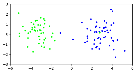
Finally, looking at the first two right singular vectors, we see that the first one does align quite well with the first dimension.
print(np.stack((V[:,0], V[:,1]), axis=-1))
[[-0.65359543 -0.03518408]
 [ 0.04389105 -0.01030089]
 [ 0.00334687 -0.01612429]
 ...
 [-0.01970281 -0.05868921]
 [-0.01982662 -0.04122036]
 [-0.00674388  0.01161806]]
\(\unlhd\)
4.8.2.2. Pseudoinverse#
The SVD leads to a natural generalization of the matrix inverse. First an observation. Recall that, to take the product of two square diagonal matrices, we simply multiply the corresponding diagonal entries. Let \(\Sigma \in \mathbb{R}^{r \times r}\) be a square diagonal matrix with diagonal entries \(\sigma_1,\ldots,\sigma_r\). If all diagonal entries are non-zero, then the matrix is invertible (since its columns then form a basis of the full space). The inverse of \(\Sigma\) in that case is simply the diagonal matrix \(\Sigma^{-1}\) with diagonal entries \(\sigma_1^{-1},\ldots,\sigma_r^{-1}\). This can be confirmed by checking the definition of the inverse
We are ready for our main definition.
DEFINITION (Pseudoinverse) Let \(A \in \mathbb{R}^{n \times m}\) be a matrix with compact SVD \(A = U \Sigma V^T\) and singular values \(\sigma_1 \geq \cdots \geq \sigma_r > 0\). A pseudoinverse \(A^+ \in \mathbb{R}^{m \times n}\) is defined as
\(\natural\)
While it is not obvious from the definition (why?), the pseudoinverse is in fact unique. To see that it is indeed a generalization of an inverse, we make a series of observations.
Observation 1: Note that, using that \(U\) has orthonormal columns,
which in general in not the identity matrix. Indeed it corresponds instead to the projection matrix onto the column space of \(A\), since the columns of \(U\) form an orthonormal basis of that linear subspace. As a result
So \(A A^+\) is not the identity matrix, but it does map the columns of \(A\) to themselves. Put differently, it is the identity map “when restricted to \(\mathrm{col}(A)\)”.
Similarly,
is the projection matrix onto the row space of \(A\), and
Observation 2: If \(A\) has full column rank \(m \leq n\), then \(r = m\). In that case, the columns of \(V\) form an orthonormal basis of all of \(\mathbb{R}^m\), i.e., \(V\) is orthogonal. Hence,
Similarly, if \(A\) has full row rank \(n \leq m\), then \(A A^+ = I_{n \times n}\).
If both cases hold, then \(n = m\), i.e., \(A\) is square, and \(\mathrm{rk}(A) = n\), i.e., \(A\) is invertible. We then get
That implies that \(A^+ = A^{-1}\) by the Existence of an Inverse Lemma (which includes uniqueness of the matrix inverse).
Observation 3: Recall that, when \(A\) is nonsingular, the system \(A \mathbf{x} = \mathbf{b}\) admits the unique solution \(\mathbf{x} = A^{-1} \mathbf{b}\). In the overdetermined case, the pseudoinverse provides a solution to the linear least squares problem.
LEMMA (Pseudoinverse and Least Squares) Let \(A \in \mathbb{R}^{n \times m}\) with \(m \leq n\). A solution to the linear least squares problem
is given by \(\mathbf{x}^* = A^+ \mathbf{b}\). Further, if \(A\) has full column rank \(m\), then
\(\flat\)
Proof idea: For the first part, we use that the solution to the least squares problem is the orthogonal projection. For the second part, we use the SVD definition and check that the two sides are the same.
Proof: Let \(A = U \Sigma V^T\) be a compact SVD of \(A\). For the first claim, note that the choice of \(\mathbf{x}^*\) in the statement gives
Hence, \(A \mathbf{x}^*\) is the orthogonal projection of \(\mathbf{b}\) onto the column space of \(A\) - which we proved previously is the solution to the linear least squares problem.
Now onto the second claim. Recall that, when \(A\) is of full rank, the matrix \(A^T A\) is nonsingular. We then note that, using the notation \(\Sigma^{-2} = (\Sigma^{-1})^2\),
as claimed. Here, we used that \((V \Sigma^2 V^T)^{-1} = V \Sigma^{-2} V^T\), which can be confirmed by checking the definition of an inverse and our previous observation about the inverse of a diagonal matrix. \(\square\)
The pseudoinverse also provides a solution in the case of an underdetermined system. Here, however, there are in general infinitely many solutions. The one chosen by the pseudoinverse has a special property as we see now: it is the least norm solution.
LEMMA (Pseudoinverse and Underdetermined Systems) Let \(A \in \mathbb{R}^{n \times m}\) with \(m > n\) and \(\mathbf{b} \in \mathbb{R}^n\). Further assume that \(A\) has full row rank \(n\). Then \(\mathbf{x}^* = A^+ \mathbf{b}\) is a solution to
Moreover, in that case,
\(\flat\)
Proof: We first prove the formula for \(A^+\). As we did in the overdetermined case, it can be checked by substituting a compact SVD \(A = U \Sigma V^T\). Recall that, when \(A^T\) is of full rank, the matrix \(A A^T\) is nonsingular. We then note that
as claimed. Here, we used that \((U \Sigma^2 U^T)^{-1} = U \Sigma^{-2} U^T\), which can be confirmed by checking the definition of an inverse and our previous observation about the inverse of a diagonal matrix.
Because \(A\) has full row rank, \(\mathbf{b} \in \mathrm{col}(A)\) and there is at least one \(\mathbf{x}\) such that \(A \mathbf{x} = \mathbf{b}\). One such solution is provided by the pseudoinverse. Indeed, from a previous observation,
where we used that the columns of \(U\) form an orthonormal basis of \(\mathbb{R}^n\) by the rank assumption.
Let \(\mathbf{x}\) be any other solution to the system. Then \(A(\mathbf{x} - \mathbf{x}^*) = \mathbf{b} - \mathbf{b} = \mathbf{0}\). That implies
In words, \(\mathbf{x} - \mathbf{x}^*\) and \(\mathbf{x}^*\) are orthogonal. By Pythagoras,
That proves that \(\mathbf{x}^*\) has the smallest norm among all solutions to the system \(A \mathbf{x} = \mathbf{b}\). \(\square\)
EXAMPLE: Continuing a previous example, let
Recall that
where
We compute the pseudoinverse. By the formula, in the rank one case, it is simply (Check this!)
\(\lhd\)
EXAMPLE: Let \(A \in \mathbb{R}^{n \times n}\) be a square nonsingular matrix. Let \(A = \sum_{j=1}^n \sigma_j \mathbf{u}_j \mathbf{v}_j^T\) be a compact SVD of \(A\), where we used the fact that the rank of \(A\) is \(n\) so it has \(n\) strictly positive singular values. We seek to compute \(\|A^{-1}\|_2\) in terms of the singular values.
Because \(A\) is invertible, \(A^+ = A^{-1}\). So we compute the pseudoinverse
The sum on the right-hand side is not quite a compact SVD of \(A^{-1}\) because the coefficients \(\sigma_j^{-1}\) are non-decreasing in \(j\).
But writing the sum in reverse order
does give a compact SVD of \(A^{-1}\), since \(\sigma_n^{-1} \geq \cdots \sigma_1^{-1} > 0\) and \(\{\mathbf{v}_j\}_{j=1}^n\) and \(\{\mathbf{u}_j\}_{j=1}^n\) are orthonormal lists. Hence, the \(2\)-norm is given by the largest singular value, that is,
\(\lhd\)
NUMERICAL CORNER: In Numpy, the pseudoinverse of a matrix can be computed using the function numpy.linalg.pinv.
M = np.array([[1.5, 1.3], [1.2, 1.9], [2.1, 0.8]])
print(M)
[[1.5 1.3]
 [1.2 1.9]
 [2.1 0.8]]
Mp = LA.pinv(M)
print(Mp)
[[ 0.09305394 -0.31101404  0.58744568]
 [ 0.12627124  0.62930858 -0.44979865]]
Mp @ M
array([[ 1.00000000e+00, -4.05255527e-17],
       [ 3.70832374e-16,  1.00000000e+00]])
Let’s try our previous example.
A = np.array([[1., 0.], [-1., 0.]])
print(A)
[[ 1.  0.]
 [-1.  0.]]
Ap = LA.pinv(A)
print(Ap)
[[ 0.5 -0.5]
 [ 0.   0. ]]
\(\unlhd\)
4.8.2.3. Condition numbers#
In this section we introduce condition numbers, a measure of perturbation sensitivity for numerical problems. We look in particular at the conditioning of the least-squares problem. We begin with the concept of pseudoinverse, which is important in its own right.
Conditioning of matrix-vector multiplication We define the condition number of a matrix and show that it captures some information about the sensitivity to perturbations of matrix-vector multiplications.
DEFINITION (Condition number of a matrix) The condition number (in the induced \(2\)-norm) of a square, nonsingular matrix \(A \in \mathbb{R}^{n \times n}\) is defined as
\(\natural\)
In fact, this can be computed as
where we used the example above. In words, \(\kappa_2(A)\) is the ratio of the largest to the smallest stretching under \(A\).
THEOREM (Conditioning of Matrix-Vector Multiplication) Let \(M \in \mathbb{R}^{n \times n}\) be nonsingular. Then, for any \(\mathbf{z} \in \mathbb{R}^n\),
and the inequality is tight in the sense that there is an \(\mathbf{x}\) and a \(\mathbf{d}\) that achieves it.
\(\sharp\)
The ratio above measures the worst rate of relative change in \(M \mathbf{z}\) under infinitesimal perturbations of \(\mathbf{z}\). The theorem says that when \(\kappa_2(M)\) is large, a case referred to as ill-conditioning, large relative changes in \(M \mathbf{z}\) can be obtained from relatively small perturbations to \(\mathbf{z}\). In words, a matrix-vector product is potentially sensitive to perturbations when the matrix is ill-conditioned.
Proof: Write
where we used \(\min_{\mathbf{u} \in \mathbb{S}^{n-1}} \|A \mathbf{u}\| = \sigma_n\), which was shown in a previous example.
In particular, we see that the ratio can achieve its maximum by taking \(\mathbf{d}\) and \(\mathbf{z}\) to be the right singular vectors corresponding to \(\sigma_1\) and \(\sigma_n\) respectively. \(\square\)
If we apply the theorem to the inverse instead, we get that the relative conditioning of the nonsingular linear system \(A \mathbf{x} = \mathbf{b}\) to perturbations in \(\mathbf{b}\) is \(\kappa_2(A)\). The latter can be large in particular when the columns of \(A\) are close to linearly dependent. This is detailed in the next example.
EXAMPLE: Let \(A \in \mathbb{R}^{n \times n}\) be nonsingular. Then, for any \(\mathbf{b} \in \mathbb{R}^n\), there exists a unique solution to \(A \mathbf{x} = \mathbf{b}\), namely,
Suppose we solve the perturbed system
for some vector \(\delta\mathbf{b}\). We use the Conditioning of Matrix-Vector Multiplication Theorem to bound the norm of \(\delta\mathbf{x}\).
Specifically, set
Then
and
So we get that
Note also that, because \((A^{-1})^{-1} = A\), we have \(\kappa_2(A^{-1}) = \kappa_2(A)\). Rearranging, we finally get
Hence the larger the condition number is, the larger the potential relative effect on the solution of the linear system is for a given relative perturbation size. \(\lhd\)
NUMERICAL CORNER: In Numpy, the condition number of a matrix can be computed using the function numpy.linalg.cond.
For example, orthogonal matrices have condition number \(1\), the lowest possible value for it (Why?). That indicates that orthogonal matrices have good numerical properties.
q = 1/np.sqrt(2)
Q = np.array([[q, q], [q, -q]])
print(Q)
[[ 0.70710678  0.70710678]
 [ 0.70710678 -0.70710678]]
LA.cond(Q)
1.0000000000000002
In contrast, matrices with nearly linearly dependent columns have large condition numbers.
eps = 1e-6
A = np.array([[q, q], [q, q+eps]])
print(A)
[[0.70710678 0.70710678]
 [0.70710678 0.70710778]]
LA.cond(A)
2828429.1245844117
Let’s look at the SVD of \(A\).
u, s, vh = LA.svd(A)
print(s)
[1.41421406e+00 4.99999823e-07]
We compute the solution to \(A \mathbf{x} = \mathbf{b}\) when \(\mathbf{b}\) is the left singular vector of \(A\) corresponding to the largest singular value. Recall that in the proof of the Conditioning of Matrix-Vector Multiplication Theorem, we showed that the worst case bound is achieved when \(\mathbf{z} = \mathbf{b}\) is right singular vector of \(M= A^{-1}\) corresponding to the lowest singular value. In a previous example, given a matrix \(A = \sum_{j=1}^n \sigma_j \mathbf{u}_j \mathbf{v}_j^T\) in compact SVD form, we derived a compact SVD for the inverse as
Here, compared to the SVD of \(A\), the order of the singular values is reversed and the roles of the left and right singular vectors are exchanged. So we take \(\mathbf{b}\) to be the top left singular vector of \(A\).
b = u[:,0]
print(b)
[-0.70710653 -0.70710703]
x = LA.solve(A,b)
print(x)
[-0.49999965 -0.5 ]
We make a small perturbation in the direction of the second right singular vector. Recall that in the proof of the Conditioning of Matrix-Vector Multiplication Theorem, we showed that the worst case is achieved when \(\mathbf{d} = \delta\mathbf{b}\) is top right singular vector of \(M = A^{-1}\). By the argument above, that is the left singular vector of \(A\) corresponding to the lowest singular value.
delta = 1e-6
bp = b + delta*u[:,1]
print(bp)
[-0.70710724 -0.70710632]
The relative change in solution is:
xp = LA.solve(A,bp)
print(xp)
[-1.91421421 0.91421356]
(LA.norm(x-xp)/LA.norm(x))/(LA.norm(b-bp)/LA.norm(b))
2828429.124665918
Note that this is exactly the condition number of \(A\).
\(\unlhd\)
Back to the least-squares problem We return to the least-squares problem
where
We showed that the solution satisfies the normal equations
Here \(A\) may not be square and invertible. We define a more general notion of condition number.
DEFINITION (Condition number of a matrix: general case) The condition number (in the induced \(2\)-norm) of a matrix \(A \in \mathbb{R}^{n \times m}\) is defined as
\(\natural\)
As we show next, the condition number of \(A^T A\) can be much larger than that of \(A\) itself.
LEMMA (Condition number of \(A^T A\)) Let \(A \in \mathbb{R}^{n \times m}\) have full column rank. The
\(\flat\)
Proof idea: We use the SVD.
Proof: Let \(A = U \Sigma V^T\) be an SVD of \(A\) with singular values \(\sigma_1 \geq \cdots \geq \sigma_m > 0\). Then
In particular the latter expression is an SVD of \(A^T A\), and hence the condition number of \(A^T A\) is
\(\square\)
NUMERICAL CORNER: We give a quick example.
A = np.array([[1., 101.],[1., 102.],[1., 103.],[1., 104.],[1., 105]])
print(A)
[[  1. 101.]
 [  1. 102.]
 [  1. 103.]
 [  1. 104.]
 [  1. 105.]]
LA.cond(A)
7503.817028686101
LA.cond(A.T @ A)
56307270.00472849
This observation – and the resulting increased numerical instability – is one of the reasons we previously developed an alternative approach to the least-squares problem. Quoting [Sol, Section 5.1]:
Intuitively, a primary reason that \(\mathrm{cond}(A^T A)\) can be large is that columns of \(A\) might look “similar” […] If two columns \(\mathbf{a}_i\) and \(\mathbf{a}_j\) satisfy \(\mathbf{a}_i \approx \mathbf{a}_j\), then the least-squares residual length \(\|\mathbf{b} - A \mathbf{x}\|_2\) will not suffer much if we replace multiples of \(\mathbf{a}_i\) with multiples of \(\mathbf{a}_j\) or vice versa. This wide range of nearly—but not completely—equivalent solutions yields poor conditioning. […] To solve such poorly conditioned problems, we will employ an alternative technique with closer attention to the column space of \(A\) rather than employing row operations as in Gaussian elimination. This strategy identifies and deals with such near-dependencies explicitly, bringing about greater numerical stability.
\(\unlhd\)
We quote without proof a theorem from [Ste, Theorem 4.2.7] which sheds further light on this issue.
THEOREM (Accuracy of Least-squares Solutions) Let \(\mathbf{x}^*\) be the solution of the least-squares problem \(\min_{\mathbf{x} \in \mathbb{R}^m} \|A \mathbf{x} - \mathbf{b}\|\). Let \(\mathbf{x}_{\mathrm{NE}}\) be the solution obtained by forming and solving the normal equations in floating-point arithmetic with rounding unit \(\epsilon_M\). Then \(\mathbf{x}_{\mathrm{NE}}\) satisfies
Let \(\mathbf{x}_{\mathrm{QR}}\) be the solution obtained from a QR factorization in the same arithmetic. Then
where \(\mathbf{r}^* = \mathbf{b} - A \mathbf{x}^*\) is the residual vector. The constants \(\gamma\) are slowly growing functions of the dimensions of the problem.
\(\sharp\)
To explain, let’s quote [Ste, Section 4.2.3] again:
The perturbation theory for the normal equations shows that \(\kappa_2^2(A)\) controls the size of the errors we can expect. The bound for the solution computed from the QR equation also has a term multiplied by \(\kappa_2^2(A)\), but this term is also multiplied by the scaled residual, which can diminish its effect. However, in many applications the vector \(\mathbf{b}\) is contaminated with error, and the residual can, in general, be no smaller than the size of that error.
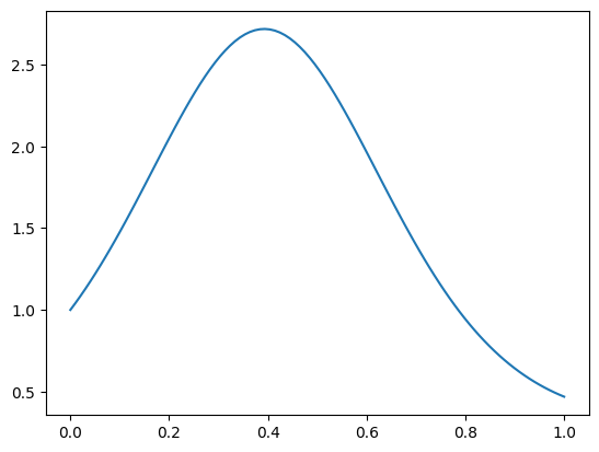
NUMERICAL CORNER: Here is a numerical example taken from [TB, Lecture 19]. We will approximate the following function with a polynomial.
n = 100
t = np.arange(n)/(n-1)
b = np.exp(np.sin(4 * t))
Show code cell source
plt.plot(t, b)
plt.show()
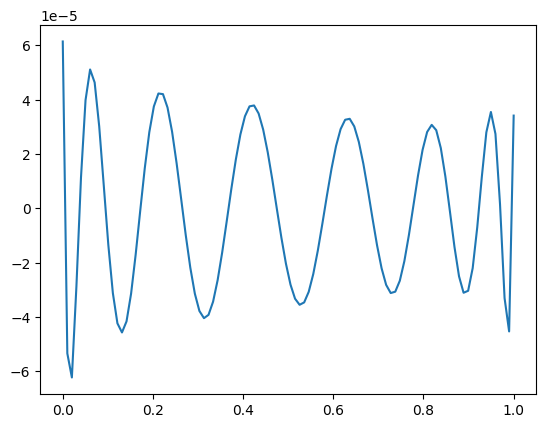
We use a Vandermonde matrix, which can be constructed using numpy.vander, to perform polynomial regression.
m = 17
A = np.vander(t, m, increasing=True)
The condition numbers of \(A\) and \(A^T A\) are both high in this case.
print(LA.cond(A))
755823354629.852
print(LA.cond(A.T @ A))
3.846226459131048e+17
We first use the normal equations and plot the residual vector.
xNE = LA.solve(A.T @ A, A.T @ b)
print(LA.norm(b - A@xNE))
0.0002873101427587512
Show code cell source
plt.plot(t, b - A@xNE)
plt.show()
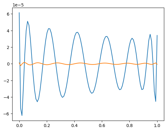
We then use numpy.linalg.qr to compute the QR solution instead.
Q, R = LA.qr(A)
xQR = mmids.backsubs(R, Q.T @ b)
print(LA.norm(b - A@xQR))
7.359657452370885e-06
Show code cell source
plt.plot(t, b - A@xNE)
plt.plot(t, b - A@xQR)
plt.show()
\(\unlhd\)
4.8.3. Additional proofs#
Proof of Greedy Finds Best Subspace In this section, we prove the full version of the Greedy Finds Best Subspace Theorem. In particular, we do not use the Spectral Theorem.
Proof idea: We proceed by induction. For an arbitrary orthonormal list \(\mathbf{w}_1,\ldots,\mathbf{w}_k\), we find an orthonormal basis of their span containing an element orthogonal to \(\mathbf{v}_1,\ldots,\mathbf{v}_{k-1}\). Then we use the defintion of \(\mathbf{v}_k\) to conclude.
Proof: We reformulate the problem as a maximization
where we also replace the \(k\)-dimensional linear subspace \(\mathcal{Z}\) with an arbitrary orthonormal basis \(\{\mathbf{w}_1,\ldots,\mathbf{w}_k\}\).
We then proceed by induction. For \(k=1\), we define \(\mathbf{v}_1\) as a solution of the above maximization problem. Assume that, for any orthonormal list \(\{\mathbf{w}_1,\ldots,\mathbf{w}_\ell\}\) with \(\ell < k\), we have
Now consider any orthonormal list \(\{\mathbf{w}_1,\ldots,\mathbf{w}_k\}\) and let its span be \(\mathcal{W} = \mathrm{span}(\mathbf{w}_1,\ldots,\mathbf{w}_k)\).
Step 1: For \(j=1,\ldots,k-1\), let \(\mathbf{v}_j'\) be the orthogonal projection of \(\mathbf{v}_j\) onto \(\mathcal{W}\) and let \(\mathcal{V}' = \mathrm{span}(\mathbf{v}'_1,\ldots,\mathbf{v}'_{k-1})\). Because \(\mathcal{V}' \subseteq \mathcal{W}\) has dimension at most \(k-1\) while \(\mathcal{W}\) itself has dimension \(k\), we can find an orthonormal basis \(\mathbf{w}'_1,\ldots,\mathbf{w}'_{k}\) of \(\mathcal{W}\) such that \(\mathbf{w}'_k\) is orthogonal to \(\mathcal{V}'\) (Why?). Then, for any \(j=1,\ldots,k-1\), we have the decomposition \(\mathbf{v}_j = \mathbf{v}'_j + (\mathbf{v}_j - \mathbf{v}'_j)\) where \(\mathbf{v}'_j \in \mathcal{V}'\) is orthogonal to \(\mathbf{w}'_k\) and \(\mathbf{v}_j - \mathbf{v}'_j\) is also orthogonal to \(\mathbf{w}'_k \in \mathcal{W}\) by the properties of the orthogonal projection onto \(\mathcal{W}\). Hence
for any \(\beta_j\)’s. That is, \(\mathbf{w}'_k\) is orthogonal to \(\mathrm{span}(\mathbf{v}_1,\ldots,\mathbf{v}_{k-1})\).
Step 2: By the induction hypothesis, we have
Moreover, recalling that the \(\boldsymbol{\alpha}_i^T\)’s are the rows of \(A\),
since the \(\mathbf{w}_j\)’s and \(\mathbf{w}'_j\)’s form an orthonormal basis of the same subspace \(\mathcal{W}\). Since \(\mathbf{w}'_k\) is orthogonal to \(\mathrm{span}(\mathbf{v}_1,\ldots,\mathbf{v}_{k-1})\) by the conclusion of Step 1, by the definition of \(\mathbf{v}_k\) as a solution to
we have
Step 3: Putting everything together
which proves the claim. \(\square\)
Proof of Existence of the SVD We return to the proof of the Existence of SVD Theorem. We give an alternative proof that does not rely on the Spectral Theorem.
Proof: We have already done most of the work. The proof works as follows:
(1) Compute the greedy sequence \(\mathbf{v}_1,\ldots,\mathbf{v}_r\) from the Greedy Finds Best Subspace Theorem until the largest \(r\) such that
or, otherwise, until \(r=m\). The \(\mathbf{v}_j\)’s are orthonormal by construction.
(2) For \(j=1,\ldots,r\), let
Observe that, by our choice of \(r\), the \(\sigma_j\)’s are \(> 0\). They are also non-increasing: by definition of the greedy sequence,
where the set of orthogonality constraints gets larger as \(i\) increases. Hence, the \(\mathbf{u}_j\)’s have unit norm by definition.
We show below that they are also orthogonal.
(3) Let \(\mathbf{z} \in \mathbb{R}^m\) be any vector. To show that our construction is correct, we prove that \(A \mathbf{z} = \left(U \Sigma V^T\right)\mathbf{z}\). Let \(\mathcal{V} = \mathrm{span}(\mathbf{v}_1,\ldots,\mathbf{v}_r)\) and decompose \(\mathbf{z}\) into orthogonal components
Applying \(A\) and using linearity, we get
We claim that \(A (\mathbf{z} - \mathrm{proj}_{\mathcal{V}}(\mathbf{z})) = \mathbf{0}\). If \(\mathbf{z} - \mathrm{proj}_{\mathcal{V}}(\mathbf{z}) = \mathbf{0}\), that is certainly the case. If not, let
By definition of \(r\),
Put differently, \(\|A \mathbf{w}_{r+1}\|^2 = 0\) (i.e. \(A \mathbf{w}_{r+1} = \mathbf{0}\)), for any unit vector \(\mathbf{w}_{r+1}\) orthogonal to \(\mathbf{v}_1,\ldots,\mathbf{v}_r\). That applies in particular to \(\mathbf{w}_{r+1} = \mathbf{w}\) by the Orthogonal Projection Theorem.
Hence, using the definition of \(\mathbf{u}_j\) and \(\sigma_j\), we get
That proves the existence of the SVD.
All that is left to prove is the orthogonality of the \(\mathbf{u}_j\)’s.
LEMMA (Left Singular Vectors are Orthogonal) For all \(1 \leq i \neq j \leq r\), \(\langle \mathbf{u}_i, \mathbf{u}_j \rangle = 0\). \(\flat\)
Proof idea: Quoting [BHK, Section 3.6]:
Intuitively if \(\mathbf{u}_i\) and \(\mathbf{u}_j\), \(i < j\), were not orthogonal, one would suspect that the right singular vector \(\mathbf{v}_j\) had a component of \(\mathbf{v}_i\) which would contradict that \(\mathbf{v}_i\) and \(\mathbf{v}_j\) were orthogonal. Let \(i\) be the smallest integer such that \(\mathbf{u}_i\) is not orthogonal to all other \(\mathbf{u}_j\). Then to prove that \(\mathbf{u}_i\) and \(\mathbf{u}_j\) are orthogonal, we add a small component of \(\mathbf{v}_j\) to \(\mathbf{v}_i\), normalize the result to be a unit vector \(\mathbf{v}'_i \propto \mathbf{v}_i + \varepsilon \mathbf{v}_j\) and show that \(\|A \mathbf{v}'_i\| > \|A \mathbf{v}_i\|\), a contradiction.
Proof: We argue by contradiction. Let \(i\) be the smallest index such that there is a \(j > i\) with \(\langle \mathbf{u}_i, \mathbf{u}_j \rangle = \delta \neq 0\). Assume \(\delta > 0\) (otherwise use \(-\mathbf{u}_i\)). For \(\varepsilon \in (0,1)\), because the \(\mathbf{v}_k\)’s are orthonormal, \(\|\mathbf{v}_i + \varepsilon \mathbf{v}_j\|^2 = 1+\varepsilon^2\). Consider the vectors
Observe that \(\mathbf{v}'_i\) is orthogonal to \(\mathbf{v}_1,\ldots,\mathbf{v}_{i-1}\), so that
On the other hand, by the Orthogonal Decomposition Lemma, we can write \(A \mathbf{v}_i'\) as a sum of its orthogonal projection on the unit vector \(\mathbf{u}_i\) and \(A \mathbf{v}_i' - \mathrm{proj}_{\mathbf{u}_i}(A \mathbf{v}_i')\), which is orthogonal to \(\mathbf{u}_i\). In particular, by Pythagoras, \(\|A \mathbf{v}_i'\| \geq \|\mathrm{proj}_{\mathbf{u}_i}(A \mathbf{v}_i')\|\). But that implies, for \(\varepsilon \in (0,1)\),
where the second inequality follows from a Taylor expansion or the observation
Now note that
for \(\varepsilon\) small enough, contradicting the inequality above. \(\square\)
SVD and Approximating Subspace In constructing the SVD of \(A\), we used the greedy sequence for the best approximating subspace. Vice versa, given an SVD of \(A\), we can read off the solution to the approximating subspace problem. In other words, there was nothing special about the specific construction we used to prove existence of the SVD. While a matrix may have many SVDs, they all give a solution to the approximating subspace problems.
Further, this perspective gives what is known as a variational characterization of the singular values. We will have more to say about variational characterizations and their uses in the next chapter.
SVD and greedy sequence Indeed, let
be an SVD of \(A\) with
We show that the \(\mathbf{v}_j\)’s form a greedy sequence for the approximating subspace problem. Complete \(\mathbf{v}_1,\ldots,\mathbf{v}_r\) into an orthonormal basis of \(\mathbb{R}^m\) by adding appropriate vectors \(\mathbf{v}_{j+1},\ldots,\mathbf{v}_m\). By construction, \(A\mathbf{v}_{i} = \mathbf{0}\) for all \(i=j+1,\ldots,m\).
We start with the case \(j=1\). For any unit vector \(\mathbf{w} \in \mathbb{R}^m\), we expand it as \(\mathbf{w} = \sum_{i=1}^m \langle \mathbf{w}, \mathbf{v}_i\rangle \,\mathbf{v}_i\). By the Properties of Orthonormal Lists,
where we used the orthonormality of the \(\mathbf{u}_i\)’s and the fact that \(\mathbf{v}_{j+1},\ldots,\mathbf{v}_m\) are in the null space of \(A\). Because the \(\sigma_i\)’s are non-increasing, this last sum is maximized by taking \(\mathbf{w} = \mathbf{v}_1\). So we have shown that \(\mathbf{v}_1 \in \arg\max\{\|A \mathbf{w}\|^2:\|\mathbf{w}\| = 1\}\).
By the Properties of Orthonormal Lists,
Hence, because the \(\sigma_i\)’s are non-increasing, the sum
This upper bound is achieved by taking \(\mathbf{w} = \mathbf{v}_1\). So we have shown that \(\mathbf{v}_1 \in \arg\max\{\|A \mathbf{w}\|^2:\|\mathbf{w}\| = 1\}\).
More generally, for any unit vector \(\mathbf{w} \in \mathbb{R}^m\) that is orthogonal to \(\mathbf{v}_1,\ldots,\mathbf{v}_{j-1}\), we expand it as \(\mathbf{w} = \sum_{i=j}^m \langle \mathbf{w}, \mathbf{v}_i\rangle \,\mathbf{v}_i\). Then, as long as \(j\leq r\),
where again we used that the \(\sigma_i\)’s are non-increasing and \(\sum_{i=1}^m \langle \mathbf{w}, \mathbf{v}_i\rangle^2 = 1\). This last bound is achieved by taking \(\mathbf{w} = \mathbf{v}_j\).
So we have shown the following.
THEOREM (Variational Characterization of Singular Values) Let \(A = \sum_{j=1}^r \sigma_j \mathbf{u}_j \mathbf{v}_j^T\) be an SVD of \(A\) with \(\sigma_1 \geq \sigma_2 \geq \cdots \geq \sigma_r > 0\). Then
and
\(\sharp\)