\(\newcommand{\bmu}{\boldsymbol{\mu}}\) \(\newcommand{\bSigma}{\boldsymbol{\Sigma}}\) \(\newcommand{\bfbeta}{\boldsymbol{\beta}}\) \(\newcommand{\bflambda}{\boldsymbol{\lambda}}\) \(\newcommand{\bgamma}{\boldsymbol{\gamma}}\) \(\newcommand{\bsigma}{{\boldsymbol{\sigma}}}\) \(\newcommand{\bpi}{\boldsymbol{\pi}}\) \(\newcommand{\btheta}{{\boldsymbol{\theta}}}\) \(\newcommand{\bphi}{\boldsymbol{\phi}}\) \(\newcommand{\balpha}{\boldsymbol{\alpha}}\) \(\newcommand{\blambda}{\boldsymbol{\lambda}}\) \(\renewcommand{\P}{\mathbb{P}}\) \(\newcommand{\E}{\mathbb{E}}\) \(\newcommand{\indep}{\perp\!\!\!\perp} \newcommand{\bx}{\mathbf{x}}\) \(\newcommand{\bp}{\mathbf{p}}\) \(\renewcommand{\bx}{\mathbf{x}}\) \(\newcommand{\bX}{\mathbf{X}}\) \(\newcommand{\by}{\mathbf{y}}\) \(\newcommand{\bY}{\mathbf{Y}}\) \(\newcommand{\bz}{\mathbf{z}}\) \(\newcommand{\bZ}{\mathbf{Z}}\) \(\newcommand{\bw}{\mathbf{w}}\) \(\newcommand{\bW}{\mathbf{W}}\) \(\newcommand{\bv}{\mathbf{v}}\) \(\newcommand{\bV}{\mathbf{V}}\) \(\newcommand{\bfg}{\mathbf{g}}\) \(\newcommand{\bfh}{\mathbf{h}}\) \(\newcommand{\horz}{\rule[.5ex]{2.5ex}{0.5pt}}\) \(\renewcommand{\S}{\mathcal{S}}\) \(\newcommand{\X}{\mathcal{X}}\) \(\newcommand{\var}{\mathrm{Var}}\) \(\newcommand{\pa}{\mathrm{pa}}\) \(\newcommand{\Z}{\mathcal{Z}}\) \(\newcommand{\bh}{\mathbf{h}}\) \(\newcommand{\bb}{\mathbf{b}}\) \(\newcommand{\bc}{\mathbf{c}}\) \(\newcommand{\cE}{\mathcal{E}}\) \(\newcommand{\cP}{\mathcal{P}}\) \(\newcommand{\bbeta}{\boldsymbol{\beta}}\) \(\newcommand{\bLambda}{\boldsymbol{\Lambda}}\) \(\newcommand{\cov}{\mathrm{Cov}}\) \(\newcommand{\bfk}{\mathbf{k}}\) \(\newcommand{\idx}[1]{}\) \(\newcommand{\xdi}{}\)

3.1. Motivating example: analyzing customer satisfaction

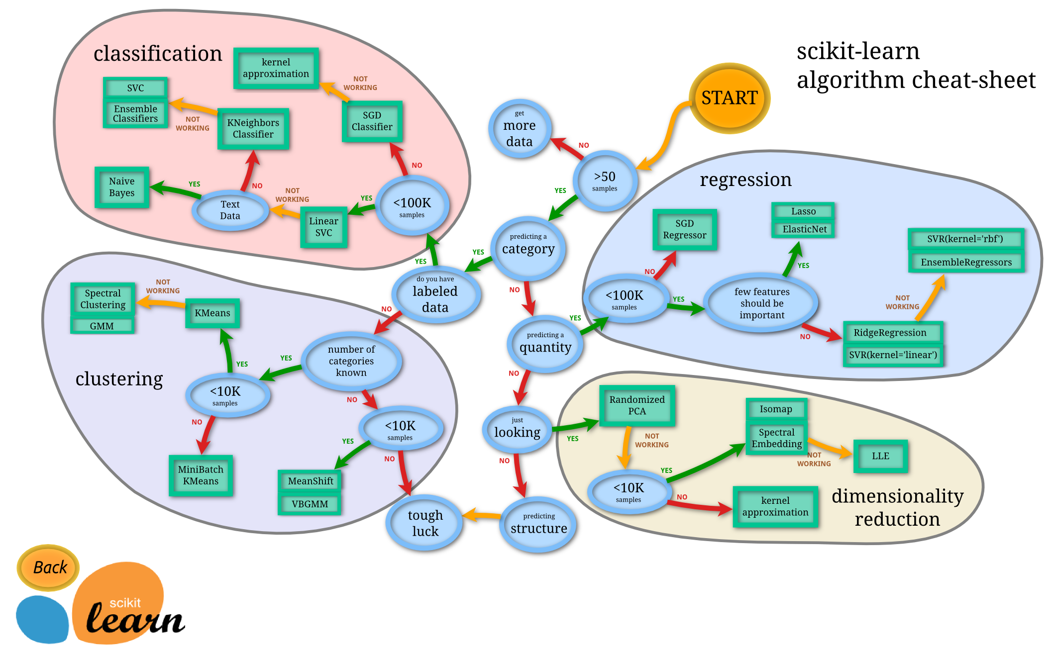
Figure: Helpful map of ML by scitkit-learn (Source)

\(\bowtie\)

We now turn to classification\(\idx{classification}\xdi\).

Quoting Wikipedia:

In machine learning and statistics, classification is the problem of identifying to which of a set of categories (sub-populations) a new observation belongs, on the basis of a training set of data containing observations (or instances) whose category membership is known. Examples are assigning a given email to the “spam” or “non-spam” class, and assigning a diagnosis to a given patient based on observed characteristics of the patient (sex, blood pressure, presence or absence of certain symptoms, etc.). Classification is an example of pattern recognition. In the terminology of machine learning, classification is considered an instance of supervised learning, i.e., learning where a training set of correctly identified observations is available.

We will illustrate this problem on an airline customer satisfaction dataset available on Kaggle, an excellent source of data and community contributed analyses. The background is the following:

The dataset consists of the details of customers who have already flown with them. The feedback of the customers on various context and their flight data has been consolidated. The main purpose of this dataset is to predict whether a future customer would be satisfied with their service given the details of the other parameters values.

We first load the data and convert it to an appropriate matrix representation. We (or, more precisely, ChatGPT) pre-processed the original file to remove rows with missing data or 0 ratings, convert categorical variables into one-hot encodings, and keep only a subset of the rows and columns. You can see the details of the pre-processing in this chat history.

data = pd.read_csv('customer_airline_satisfaction.csv')

This is a large dataset. Here are the first five rows and first 6 colums.

print(data.iloc[:5, :6])

   Satisfied  Age  Class_Business  Class_Eco  Class_Eco Plus  Business travel
0          0   63               1          0               0                1
1          0   34               1          0               0                1
2          0   52               0          1               0                0
3          0   40               0          1               0                1
4          1   46               0          1               0                1

It has 100,000 rows and 24 columns.

data.shape

(100000, 24)

The column names are:

print(data.columns.tolist())

['Satisfied', 'Age', 'Class_Business', 'Class_Eco', 'Class_Eco Plus', 'Business travel', 'Loyal customer', 'Flight Distance', 'Departure Delay in Minutes', 'Arrival Delay in Minutes', 'Seat comfort', 'Departure/Arrival time convenient', 'Food and drink', 'Gate location', 'Inflight wifi service', 'Inflight entertainment', 'Online support', 'Ease of Online booking', 'On-board service', 'Leg room service', 'Baggage handling', 'Checkin service', 'Cleanliness', 'Online boarding']

The first column indicates whether a customer was satisfied (with 1 meaning satisfied). The next 6 columns give some information about the customers, e.g., their age or whether they are members of a loyalty program with the airline. The following three columns give information about the flight, with names that should be self-explanatory: Flight Distance, Departure Delay in Minutes, and Arrival Delay in Minutes. The remaining columns give the customers’ ratings, between 1 and 5, of various feature, e.g., Baggage handling, Checkin service.

Our goal will be to predict the first column, Satisfied, from the rest of the columns. For this, we transform our data into Numpy arrays.

y = data['Satisfied'].to_numpy()
X = data.drop(columns=['Satisfied']).to_numpy()
print(y)

[0 0 0 ... 0 1 0]

print(X)

[[63  1  0 ...  3  3  4]
 [34  1  0 ...  2  3  4]
 [52  0  1 ...  4  3  4]
 ...
 [39  0  1 ...  4  1  1]
 [25  0  0 ...  5  3  1]
 [44  1  0 ...  1  2  2]]

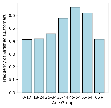
Some features may affect satisfication more than others. Let us look at age for instance. The following code extracts the Age column from X (i.e., column \(0\)) and computes the fraction of satisfied customers in several age bins.

Explanation by ChatGPT (who wrote the code):

1. numpy.digitize bins the age data into the specified age bins. The -1 adjustment is to match zero-based indexing.

2. numpy.bincount counts the occurrences of each bin index. The minlength parameter ensures that the resulting array length matches the number of age bins (age_labels). This is important if some bins have zero counts, ensuring the counts array covers all bins.

3. freq_satisfied = counts_satisfied / counts_all calculates the satisfaction frequency for each age group by dividing the counts of satisfied customers by the total counts in each age group.

age_col_index = 0
age_data = X[:, age_col_index]
age_bins = [0, 18, 25, 35, 45, 55, 65, 100]
age_labels = ['0-17', '18-24', '25-34', '35-44', '45-54', '55-64', '65+']
age_bin_indices = np.digitize(age_data, bins=age_bins) - 1
counts_all = np.bincount(age_bin_indices, minlength=len(age_labels))
counts_satisfied = np.bincount(age_bin_indices[y == 1], minlength=len(age_labels))
freq_satisfied = counts_satisfied / counts_all
age_group_labels = np.array(age_labels)

The results are plotted using matplotlib’s matplotlib.pyplot.bar function. We see in particular that younger people tend to be more dissatisfied. Of course, this might be because they cannot afford the most expensive services.

plt.figure(figsize=(4, 4))
plt.bar(age_group_labels, freq_satisfied, color='lightblue', edgecolor='black')
plt.xlabel('Age Group'), plt.ylabel('Frequency of Satisfied Customers')
plt.show()

The input data is now of the form \(\{(\mathbf{x}_i, y_i) : i=1,\ldots, n\}\) where \(\mathbf{x}_i \in \mathbb{R}^d\) are the features and \(y_i \in \{0,1\}\) is the label. Above we use the matrix representation \(X \in \mathbb{R}^{d \times n}\) with columns \(\mathbf{x}_i\), \(i = 1,\ldots, n\) and \(\mathbf{y} = (y_1, \ldots, y_n)^T \in \{0,1\}^n\).

Our goal:

learn a classifier from the examples \(\{(\mathbf{x}_i, y_i) : i=1,\ldots, n\}\), that is, a function \(\hat{f} : \mathbb{R}^d \to \mathbb{R}\) such that \(\hat{f}(\mathbf{x}_i) \approx y_i\).

We may want to enforce that the output is in \(\{0,1\}\) as well. This problem is referred to as binary classification.

A natural approach to this type of supervised learning\(\idx{supervised learning}\xdi\) problem is to define two objects:

1. Family of classifiers: A class \(\widehat{\mathcal{F}}\) of classifiers from which to pick \(\hat{f}\).

2. Loss function: A loss function \(\ell(\hat{f}, (\mathbf{x},y))\) which quantifies how good of a fit \(\hat{f}(\mathbf{x})\) is to \(y\).

Our goal is then to solve

\[ \min_{\hat{f} \in \widehat{\mathcal{F}}} \frac{1}{n} \sum_{i=1}^n \ell(\hat{f}, (\mathbf{x}_i, y_i)), \]

that is, we seek to find a classifier among \(\widehat{\mathcal{F}}\) that minimizes the average loss over the examples.

For instance, in logistic regression, we consider linear classifiers of the form

\[ \hat{f}(\mathbf{x}) = \sigma(\mathbf{x}^T \boldsymbol{\theta}) \qquad \text{with} \qquad \sigma(t) = \frac{1}{1 + e^{-t}} \]

where \(\boldsymbol{\theta} \in \mathbb{R}^d\) is a parameter vector. And we use the cross-entropy loss

\[ \ell(\hat{f}, (\mathbf{x}, y)) = - y \log(\sigma(\mathbf{x}^T \boldsymbol{\theta})) - (1-y) \log(1- \sigma(\mathbf{x}^T \boldsymbol{\theta})). \]

In parametric form, the problem boils down to

\[ \min_{\boldsymbol{\theta} \in \mathbb{R}^d} - \frac{1}{n} \sum_{i=1}^n y_i \log(\sigma(\mathbf{x}_i^T \boldsymbol{\theta})) - \frac{1}{n} \sum_{i=1}^n (1-y_i) \log(1- \sigma(\mathbf{x}_i^T \boldsymbol{\theta})). \]

To obtain a prediction in \(\{0,1\}\) here, we could cutoff \(\hat{f}(\mathbf{x})\) at a threshold \(\tau \in [0,1]\), that is, return \(\mathbf{1}\{\hat{f}(\mathbf{x}) > \tau\}\).

We will explain in a later chapter where this choice comes from.

The purpose of this chapter is to develop some of the mathematical theory and algorithms needed to solve this type of optimization formulation.

CHAT & LEARN Ask your favorite AI chatbot to help you explore the following hypothesis about this dataset:

Younger people tend to be more dissatisfied because they cannot afford the best services.

For example, consider the relationship between age, satisfaction, and class (e.g., economy, business, etc.). Specifically:

1. Compare the distribution of class types among different age groups.

2. Compare the satisfaction levels within each class type for different age groups.

(Open In Colab) \(\ddagger\)