
\(\newcommand{\bmu}{\boldsymbol{\mu}}\) \(\newcommand{\bSigma}{\boldsymbol{\Sigma}}\) \(\newcommand{\bfbeta}{\boldsymbol{\beta}}\) \(\newcommand{\bflambda}{\boldsymbol{\lambda}}\) \(\newcommand{\bgamma}{\boldsymbol{\gamma}}\) \(\newcommand{\bsigma}{{\boldsymbol{\sigma}}}\) \(\newcommand{\bpi}{\boldsymbol{\pi}}\) \(\newcommand{\btheta}{{\boldsymbol{\theta}}}\) \(\newcommand{\bphi}{\boldsymbol{\phi}}\) \(\newcommand{\balpha}{\boldsymbol{\alpha}}\) \(\newcommand{\blambda}{\boldsymbol{\lambda}}\) \(\renewcommand{\P}{\mathbb{P}}\) \(\newcommand{\E}{\mathbb{E}}\) \(\newcommand{\indep}{\perp\!\!\!\perp} \newcommand{\bx}{\mathbf{x}}\) \(\newcommand{\bp}{\mathbf{p}}\) \(\renewcommand{\bx}{\mathbf{x}}\) \(\newcommand{\bX}{\mathbf{X}}\) \(\newcommand{\by}{\mathbf{y}}\) \(\newcommand{\bY}{\mathbf{Y}}\) \(\newcommand{\bz}{\mathbf{z}}\) \(\newcommand{\bZ}{\mathbf{Z}}\) \(\newcommand{\bw}{\mathbf{w}}\) \(\newcommand{\bW}{\mathbf{W}}\) \(\newcommand{\bv}{\mathbf{v}}\) \(\newcommand{\bV}{\mathbf{V}}\) \(\newcommand{\bfg}{\mathbf{g}}\) \(\newcommand{\bfh}{\mathbf{h}}\) \(\newcommand{\horz}{\rule[.5ex]{2.5ex}{0.5pt}}\) \(\renewcommand{\S}{\mathcal{S}}\) \(\newcommand{\X}{\mathcal{X}}\) \(\newcommand{\var}{\mathrm{Var}}\) \(\newcommand{\pa}{\mathrm{pa}}\) \(\newcommand{\Z}{\mathcal{Z}}\) \(\newcommand{\bh}{\mathbf{h}}\) \(\newcommand{\bb}{\mathbf{b}}\) \(\newcommand{\bc}{\mathbf{c}}\) \(\newcommand{\cE}{\mathcal{E}}\) \(\newcommand{\cP}{\mathcal{P}}\) \(\newcommand{\bbeta}{\boldsymbol{\beta}}\) \(\newcommand{\bLambda}{\boldsymbol{\Lambda}}\) \(\newcommand{\cov}{\mathrm{Cov}}\) \(\newcommand{\bfk}{\mathbf{k}}\) \(\newcommand{\idx}[1]{}\) \(\newcommand{\xdi}{}\)
4.5. Application: principal components analysis#
We discuss an application to principal components analysis and revisit our genetic dataset from ealier in the chapter.
4.5.1. Dimensionality reduction via principal components analysis (PCA)#
Principal components analysis (PCA)\(\idx{principal components analysis}\xdi\) is a commonly used dimensionality reduction approach that is closely related to what we described in the previous sections. We formalize the connection.
The data matrix: In PCA we are given \(n\) data points \(\mathbf{x}_1,\ldots,\mathbf{x}_n \in \mathbb{R}^p\) with \(p\) features (i.e., coordinates). We denote the components of \(\mathbf{x}_i\) as \((x_{i1},\ldots,x_{ip})\). As usual, we stack them up into a matrix \(X\) whose \(i\)-th row is \(\mathbf{x}_i^T\).
The first step of PCA is to center the data, i.e., we assume that\(\idx{mean centering}\xdi\)
Put differently, the empirical mean of each column is \(0\). Quoting Wikipedia (and this will become clearer below):
Mean subtraction (a.k.a. “mean centering”) is necessary for performing classical PCA to ensure that the first principal component describes the direction of maximum variance. If mean subtraction is not performed, the first principal component might instead correspond more or less to the mean of the data. A mean of zero is needed for finding a basis that minimizes the mean square error of the approximation of the data.
An optional step is to divide each column by the square root of its sample variance, i.e., assume that
As we mentioned in a previous chapter, this is particularly important when the features are measured in different units to ensure that their variability can be meaningfully compared.
The first principal component: The first principal component is the linear combination of the features
with largest sample variance. For this to make sense, we need to constrain the \(\phi_{j1}\)s. Specifically, we require
The \(\phi_{j1}\)s are referred to as the loadings and the \(t_{i1}\)s are referred to as the scores.
Formally, we seek to solve
where we used the fact that the \(t_{i1}\)s are centered
to compute their sample variance as the mean of their square
Let \(\boldsymbol{\phi}_1 = (\phi_{11},\ldots,\phi_{p1})\) and \(\mathbf{t}_1 = (t_{11},\ldots,t_{n1})\). Then for all \(i\)
or in vector form
Also
Rewriting the maximization problem above in vector form,
we see that we have already encountered this problem (up to the factor of \(1/(n-1)\) which does not affect the solution). The solution is to take \(\boldsymbol{\phi}_1\) to be the top right singular vector of \(\frac{1}{\sqrt{n-1}}X\) (or simply \(X\)). As we know this is equivalent to computing the top eigenvector of the matrix \(\frac{1}{n-1} X^T X\), which is the sample covariance matrix of the data (accounting for the fact that the data is already centered).
The second principal component: The second principal component is the linear combination of the features
with largest sample variance that is also uncorrelated with the first principal component, in the sense that
The next lemma shows how to deal with this condition. Again, we also require
As before, let \(\boldsymbol{\phi}_2 = (\phi_{12},\ldots,\phi_{p2})\) and \(\mathbf{t}_2 = (t_{12},\ldots,t_{n2})\).
LEMMA (Uncorrelated Principal Components) Assume \(X \neq \mathbf{0}\). Let \(t_{i1}\), \(t_{i2}\), \(\boldsymbol{\phi}_1\), \(\boldsymbol{\phi}_2\) be as above (where, in particular, \(\boldsymbol{\phi}_1\) is a top right singular vector of \(X\)). Then
holds if and only if
\(\flat\)
Proof: The condition
is equivalent to
where we dropped the \(1/(n-1)\) factor as it does not play any role. Using that \(\mathbf{t}_1 = X \boldsymbol{\phi}_1\), and similarly, \(\mathbf{t}_2 = X \boldsymbol{\phi}_2\), this is in turn equivalent to
Because \(\boldsymbol{\phi}_1\) can be chosen as a top right singular vector in an SVD of \(X\), it follows from the SVD Relations that \(X^T X \boldsymbol{\phi}_1 = \sigma_1^2 \boldsymbol{\phi}_1\), where \(\sigma_1\) is the singular value associated to \(\boldsymbol{\phi}_1\). Since \(X \neq 0\), \(\sigma_1 > 0\). Plugging this in the inner product on the left hand side above, we get
Because \(\sigma_1 \neq 0\), this is \(0\) if and only if \(\langle \boldsymbol{\phi}_1, \boldsymbol{\phi}_2 \rangle = 0\). \(\square\)
As a result, we can write the maximization problem for the second principal component in matrix form as
Again, we see that we have encountered this problem before. The solution is to take \(\boldsymbol{\phi}_2\) to be a second right singular vector in an SVD of \(\frac{1}{\sqrt{n-1}}X\) (or simply \(X\)). Again, this is equivalent to computing the second eigenvector of the sample covariance matrix \(\frac{1}{n-1} X^T X\).
Further principal components: We can proceed in a similar fashion and define further principal components.
To quote Wikipedia:
PCA essentially rotates the set of points around their mean in order to align with the principal components. This moves as much of the variance as possible (using an orthogonal transformation) into the first few dimensions. The values in the remaining dimensions, therefore, tend to be small and may be dropped with minimal loss of information […] PCA is often used in this manner for dimensionality reduction. PCA has the distinction of being the optimal orthogonal transformation for keeping the subspace that has largest “variance” […]
Formally, let
be the SVD of the data matrix \(X\). The principal component transformation, truncated at the \(\ell\)-th component, is
where \(T\) is the matrix whose columns are the vectors \(\mathbf{t}_1,\ldots,\mathbf{t}_\ell\). Recall that \(V_{(\ell)}\) is the matrix made of the first \(k\) columns of \(V\).
Then, using the orthonormality of the right singular vectors,
Put differently, the vector \(\mathbf{t}_i\) is the left singular vector \(\mathbf{u}_i\) scaled by the corresponding singular value \(\sigma_i\).
Having established a formal connection between PCA and SVD, we implement PCA using the SVD algorithm numpy.linalg.svd. We perform mean centering (now is the time to read that quote about the importance of mean centering again), but not the optional standardization. We use the fact that, in NumPy, subtracting a matrix by a vector whose dimension matches the number of columns performs row-wise subtraction.
def pca(X, l):
    mean = np.mean(X, axis=0)
    Y = X - mean
    U, S, Vt = LA.svd(Y, full_matrices=False)
    return U[:, :l] @ np.diag(S[:l])
NUMERICAL CORNER: We apply it to the Gaussian Mixture Model.
seed = 535
rng = np.random.default_rng(seed)
d, n, w = 1000, 100, 3.
X = mmids.two_mixed_clusters(rng, d, n, w)
T = pca(X, 2)
Plotting the result, we see that PCA does succeed in finding the main direction of variation. Note tha gap in the middle.
fig = plt.figure()
ax = fig.add_subplot(111,aspect='equal')
ax.scatter(T[:,0], T[:,1], s=5, c='k')
plt.show()
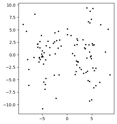
Note however that the first two principal components in fact “capture more noise” than what can be seen in the orginal first two coordinates, a form of overfitting.
TRY IT! Compute the first two right singular vectors \(\mathbf{v}_1\) and \(\mathbf{v}_2\) of \(X\) after mean centering. Do they align well with the first and second standard basis vectors \(\mathbf{e}_1\) and \(\mathbf{e}_2\)? Why or why not? (Open in Colab)
\(\unlhd\)
We return to our motivating example. We apply PCA to our genetic dataset.
Figure: Viruses (Credit: Made with Midjourney)

\(\bowtie\)
NUMERICAL CORNER: We load the dataset again. Recall that it contains \(1642\) strains and lives in a \(317\)-dimensional space.
data = pd.read_csv('h3n2-snp.csv')
Our goal is to find a “good” low-dimensional representation of the data. We work with ten dimensions using PCA.
A = data[[data.columns[i] for i in range(1,len(data.columns))]].to_numpy()
n_dims = 10
T = pca(A, n_dims)
We plot the first two principal components, and see what appears to be some potential structure.
plt.figure(figsize=(5,3))
plt.scatter(T[:,0], T[:,1], s=10, c='k')
plt.axis([-3,6,-3,3])
plt.show()
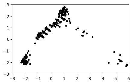
There seems to be some reasonably well-defined clusters in this projection. We use \(k\)-means to identiy clusters. We take advantage of the implementation in scikit-learn, sklearn.cluster.KMeans. By default, it finds \(8\) clusters. The clusters can be extracted from the attribute labels_.
from sklearn.cluster import KMeans

n_clusters = 8
kmeans = KMeans(n_clusters=n_clusters, init='k-means++',
                random_state=seed, n_init=10).fit(T)
assign = kmeans.labels_
To further reveal the structure, we look at our the clusters spread out over the years. That information is in a separate file.
data_oth = pd.read_csv('h3n2-other.csv')
data_oth.head()
| strain | length | country | year | lon | lat | date | |
|---|---|---|---|---|---|---|---|
| 0 | AB434107 | 1701 | Japan | 2002 | 137.215474 | 35.584176 | 2002/02/25 |
| 1 | AB434108 | 1701 | Japan | 2002 | 137.215474 | 35.584176 | 2002/03/01 |
| 2 | CY000113 | 1762 | USA | 2002 | -73.940000 | 40.670000 | 2002/01/29 |
| 3 | CY000209 | 1760 | USA | 2002 | -73.940000 | 40.670000 | 2002/01/17 |
| 4 | CY000217 | 1760 | USA | 2002 | -73.940000 | 40.670000 | 2002/02/26 |
year = data_oth['year'].to_numpy()
For each cluster, we plot how many of its data points come from a specific year. Each cluster has a different color.
fig, ax = plt.subplots(figsize=(6,4))

for i in range(n_clusters):
    unique, counts = np.unique(year[assign == i], return_counts=True)
    ax.bar(unique, counts, label=i)

ax.set(xlim=(2001, 2007), xticks=np.arange(2002, 2007))
ax.legend()
plt.show()
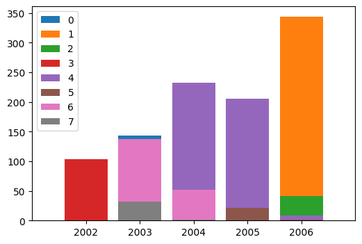
Remarkably, we see that each cluster comes mostly from one year or two consecutive ones. In other words, the clustering in this low-dimensional projection captures some true underlying structure that is not explicitly in the genetic data on which it is computed.
Going back to the first two principal components, we color the points on the scatterplot by year. (We use legend_elements() for automatic legend creation.)
fig = plt.figure(figsize=(5,3))
ax = fig.add_subplot(111, aspect='equal')
scatter = ax.scatter(T[:,0], T[:,1], s=10,  c=year, label=year)
plt.legend(*scatter.legend_elements())
plt.show()
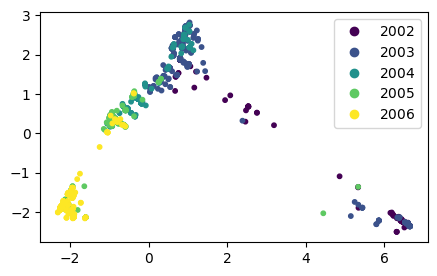
To some extent, one can “see” the virus evolving from year to year. The \(x\)-axis in particular seems to correlate strongly with the year, in the sense that samples from later years tend to be towards one side of the plot.
To further quantify this observation, we use numpy.corrcoef to compute the correlation coefficients between the year and the first \(10\) principal components.
corr = np.zeros(n_dims)
for i in range(n_dims):
    corr[i] = np.corrcoef(np.stack((T[:,i], year)))[0,1]

print(corr)
[-0.7905001  -0.42806325  0.0870437  -0.16839491  0.05757342 -0.06046913
 -0.07920042  0.01436618 -0.02544749  0.04314641]
Indeed, we see that the first three or four principal components correlate well with the year.
Using related techniques, one can also identify which mutations distinguish different epidemics (i.e., years).
\(\unlhd\)
CHAT & LEARN Ask your favorite AI chatbot about the difference between principal components analysis (PCA) and linear discriminant analysis (LDA). \(\ddagger\)
Self-assessment quiz (with help from Claude, Gemini, and ChatGPT)
1 What is the goal of principal components analysis (PCA)?
a) To find clusters in the data.
b) To find a low-dimensional representation of the data that captures the maximum variance.
c) To find the mean of each feature in the data.
d) To find the correlation between features in the data.
2 Formally, the first principal component is the linear combination of features \(t_{i1} = \sum_{j=1}^p \phi_{j1} x_{ij}\) that solves which optimization problem?
a) \(\max \left\{ \frac{1}{n-1} \|X\boldsymbol{\phi}_1\|^2 : \|\boldsymbol{\phi}_1\|^2 = 1\right\}\)
b) \(\min \left\{ \frac{1}{n-1} \|X\boldsymbol{\phi}_1\|^2 : \|\boldsymbol{\phi}_1\|^2 = 1\right\}\)
c) \(\max \left\{ \frac{1}{n-1} \|X\boldsymbol{\phi}_1\|^2 : \|\boldsymbol{\phi}_1\|^2 \leq 1\right\}\)
d) \(\min \left\{ \frac{1}{n-1} \|X\boldsymbol{\phi}_1\|^2 : \|\boldsymbol{\phi}_1\|^2 \leq 1\right\}\)
3 What is the relationship between the loadings in PCA and the singular vectors of the data matrix?
a) The loadings are the left singular vectors.
b) The loadings are the right singular vectors.
c) The loadings are the singular values.
d) There is no direct relationship between loadings and singular vectors.
4 What is the dimensionality of the matrix \(T\) in the principal component transformation \(T = XV^{(l)}\)?
a) \(n \times p\)
b) \(n \times l\)
c) \(l \times p\)
d) \(p \times l\)
5 What is the purpose of centering the data in PCA?
a) To make the calculations easier.
b) To ensure the first principal component describes the direction of maximum variance.
c) To normalize the data.
d) To remove outliers.
Answer for 1: b. Justification: The text states that “Principal components analysis (PCA) is a commonly used dimensionality reduction approach” and that “The first principal component is the linear combination of the features … with largest sample variance.”
Answer for 2: a. Justification: The text states that “Formally, we seek to solve \(\max \left\{ \frac{1}{n-1} \|X\boldsymbol{\phi}_1\|^2 : \|\boldsymbol{\phi}_1\|^2 = 1\right\}\).”
Answer for 3: b. Justification: The text explains that the solution to the PCA optimization problem is to take the loadings to be the top right singular vector of the data matrix.
Answer for 4: b. Justification: The matrix \(T\) contains the scores of the data points on the first \(l\) principal components. Since there are \(n\) data points and \(l\) principal components, the dimensionality of \(T\) is \(n \times l\).
Answer for 5: b. Justification: The text mentions that “Mean subtraction (a.k.a. ‘mean centering’) is necessary for performing classical PCA to ensure that the first principal component describes the direction of maximum variance.”