\(\newcommand{\P}{\mathbb{P}}\) \(\newcommand{\E}{\mathbb{E}}\) \(\newcommand{\S}{\mathcal{S}}\) \(\newcommand{\var}{\mathrm{Var}}\) \(\newcommand{\bmu}{\boldsymbol{\mu}}\) \(\newcommand{\bSigma}{\boldsymbol{\Sigma}}\) \(\newcommand{\btheta}{\boldsymbol{\theta}}\) \(\newcommand{\bpi}{\boldsymbol{\pi}}\) \(\newcommand{\indep}{\perp\!\!\!\perp}\) \(\newcommand{\bp}{\mathbf{p}}\) \(\newcommand{\bx}{\mathbf{x}}\) \(\newcommand{\bX}{\mathbf{X}}\) \(\newcommand{\by}{\mathbf{y}}\) \(\newcommand{\bY}{\mathbf{Y}}\) \(\newcommand{\bz}{\mathbf{z}}\) \(\newcommand{\bZ}{\mathbf{Z}}\) \(\newcommand{\bw}{\mathbf{w}}\) \(\newcommand{\bW}{\mathbf{W}}\) \(\newcommand{\bv}{\mathbf{v}}\) \(\newcommand{\bV}{\mathbf{V}}\) \(\newcommand{\bLambda}{\boldsymbol{\Lambda}}\) \(\newcommand{\bu}{\mathbf{u}}\) \(\newcommand{\bU}{\mathbf{U}}\)
7.4. Linear-Gaussian models and Kalman filtering#
In this section, we illustrate the use of linear-Gaussian models for object tracking. We first give some background.
7.4.1. Multivariate Gaussians: marginals and conditionals#
We will need the marginal and conditional densities of a multivariate Gaussian. We first need various formulas and results about block matrices.
Block matrices It will be convenient to introduce block matrices. First recall that, for a vector \(\mathbf{x} \in \mathbb{R}^n\), we write \(\mathbf{x} = (\mathbf{x}_1, \mathbf{x}_2)\), where \(\mathbf{x}_1 \in \mathbb{R}^{n_1}\) and \(\mathbf{x}_2 \in \mathbb{R}^{n_2}\) with \(n_1 + n_2 = n\), to indicate that \(\mathbf{x}\) is partitioned into two blocks: \(\mathbf{x}_1\) corresponds to the first \(n_1\) coordinates of \(\mathbf{x}\) while \(\mathbf{x}_2\) corresponds to the following \(n_2\) coordinates.
More generally, a block matrix is a partitioning of the rows and columns of a matrix of the form
where \(A \in \mathbb{R}^{n \times m}\), \(A_{ij} \in \mathbb{R}^{n_i \times m_j}\) for \(i,j = 1, 2\) with the conditions \(n_1 + n_2 = n\) and \(m_1 + m_2 = m\). One can also consider larger numbers of blocks, but it will not be necessary here.
Block matrices have a convenient algebra that mimics the usual matrix algebra. Specifically, if \(B_{ij} \in \mathbb{R}^{m_i \times p_j}\) for \(i,j = 1, 2\), then it holds that
Observe that the block sizes of \(A\) and \(B\) must match for this formula to make sense. You can convince yourself of this identity by trying it on a simple example. For a proof sketch, see e.g. here. Warning: while the formula is similar to the usual matrix product, the order of multiplication matters because the blocks are matrices and they do not in general commute!
Consider a square block matrix with the same partitioning of the rows and columns, that is,
where \(A \in \mathbb{R}^{n \times n}\), \(A_{ij} \in \mathbb{R}^{n_i \times n_i}\) for \(i = 1, 2\) with the condition \(n_1 + n_2 = n\). Then it is straightforward to check (try it!) that the transpose can be written as
In particular, if \(A\) is symmetric then \(A_{11} = A_{11}^T\), \(A_{22} = A_{22}^T\) and \(A_{21} = A_{12}^T\).
EXAMPLE: The formula above applies to partitioned vectors as well by taking for instance \(B_{11}\) and \(B_{22}\) to be empty blocks. For instance, consider the \(\mathbf{z} = (\mathbf{z}_1, \mathbf{z}_2)\), where \(\mathbf{z}_1 \in \mathbb{R}^{n_1}\) and \(\mathbf{z}_2 \in \mathbb{R}^{n_2}\). We want to compute the quadratic form
where \(A_{ij} \in \mathbb{R}^{n_i \times n_j}\) for \(i,j = 1, 2\) with the conditions \(n_1 + n_2 = n\), and \(A_{11}^T = A_{11}\) and \(A_{22}^T = A_{22}\).
We apply the formula above twice to get
\(\lhd\)
EXAMPLE: Let \(A_{ii} \in \mathbb{R}^{n_i \times n_i}\) for \(i = 1, 2\) be invertible. We claim that
The matrix on the right-hand side is well-defined by the invertibility of \(A_{11}\) and \(A_{22}\). We check the claim using the formula for matrix products of block matrices. The matrices above are block diagonal.
Indeed, we obtain
and similarly for the other direction. \(\lhd\)
EXAMPLE: Let \(A_{21} \in \mathbb{R}^{n_2 \times n_1}\). Then we claim that
A similar formula holds for the block upper triangular case. In particular, such matrices are invertible (which can be proved in other ways, for instance through determinants).
It suffices to check:
Taking a transpose gives a similar formula for the block upper triangular case. \(\lhd\)
Schur complement We will need the concept of a Schur complement. We start with a couple observations about positive definite matrices.
Recall:
LEMMA (Invertibility of Positive Definite Matrices) Let \(B \in \mathbb{R}^{n \times n}\) be positive definite. Then \(B\) is invertible. \(\flat\)
Proof: For any \(\mathbf{x} \neq \mathbf{0}\), it holds by positive definiteness that \(\mathbf{x}^T B \mathbf{x} > 0\). In particular, it must be that \(\mathbf{x}^T B \mathbf{x} \neq 0\) and therefore, by contradiction, \(B \mathbf{x} \neq \mathbf{0}\) (since for any \(\mathbf{z}\), it holds that \(\mathbf{z}^T \mathbf{0} = 0\)). The claim follows from the Equivalent Definition of Linear Independence. \(\square\)
A principal submatrix is a square submatrix obtained by removing some rows and columns. Moreover we require that the set of row indices that remain is the same as the set of column indices that remain.
LEMMA (Principal Submatrices) Let \(B \in \mathbb{R}^{n \times n}\) be positive definite and let \(Z \in \mathbb{R}^{n \times p}\) have full column rank. Then \(Z^T B Z\) is positive definite. In particular all principal submatrices of positive definite matrices are positive definite. \(\flat\)
Proof: If \(\mathbf{x} \neq \mathbf{0}\), then \(\mathbf{x}^T (Z^T B Z) \mathbf{x} = \mathbf{y}^T B \mathbf{y}\), where we defined \(\mathbf{y} = Z \mathbf{x}\). Because \(Z\) has full column rank and \(\mathbf{x} \neq \mathbf{0}\), it follows that \(\mathbf{y} \neq \mathbf{0}\) by the Equivalent Definition of Linear Independence. Hence, since \(B \succ 0\), we have \(\mathbf{y}^T B \mathbf{y} > 0\) which proves the first claim. For the second claim, take \(Z\) of the form \((\mathbf{e}_{m_1}\ \mathbf{e}_{m_2}\ \ldots\ \mathbf{e}_{m_p})\), where the indices \(m_1, \ldots, m_p\) are distinct and increasing. The columns of \(Z\) are then linearly independent since they are distinct basis vectors. \(\square\)
To better understand the last claim in the proof, note that
So if the \(i\)-th column of \(Z\) is \(\mathbf{e}_{m_i}\) and the \(j\)-th column of \(Z\) is \(\mathbf{e}_{m_j}\), then the rightmost summation picks up only one element, \(B_{m_i, m_j}\). In other words, \(Z^T B Z\) is the principal submatrix of \(B\) corresponding to rows and columns \(m_1, \ldots, m_p\).
MULTIPLE CHOICE: Consider the matrices
Which of the following matrices is \(Z^T A Z\)?
a) \(\begin{pmatrix} 1 & 0\\ 6 & 1 \end{pmatrix}\)
b) \(\begin{pmatrix} 8 & 0\\ 2 & 1 \end{pmatrix}\)
c) \(\begin{pmatrix} 2 & 8 & 4 & 0\\ 3 & 2 & 0 & 1 \end{pmatrix}\)
d) \(\begin{pmatrix} 1 & 0\\ 2 & 4\\ 6 & 1\\ 3 & 0 \end{pmatrix}\)
\(\ddagger\)
LEMMA (Schur Complement) Let \(B \in \mathbb{R}^{n \times n}\) be positive definite and write it in block form
where \(B_{11} \in \mathbb{R}^{n_1 \times n_1}\) and \(B_{22} \in \mathbb{R}^{n - n_1 \times n - n_1}\) are symmetric, and \(B_{12} \in \mathbb{R}^{n_1 \times n - n_1}\) . Then the Schur complement of the block \(B_{11}\), i.e., the matrix \(B/B_{11} := B_{22} - B_{12}^T B_{11}^{-1} B_{12}\), is symmetric and positive definite. The same holds for \(B/B_{22} := B_{11} - B_{12} B_{22}^{-1} B_{12}^T\). \(\flat\)
Proof: By the Principal Submatrices Lemma, \(B_{11}\) is positive definite. By the Invertibility of Positive Definite Matrices Lemma, \(B_{11}\) is therefore invertible. Hence the Schur complement is well defined. Moreover, it is symmetric since
by the symmetry of \(B_{11}\), \(B_{22}\), and \(B_{11}^{-1}\) (prove that last one!).
For a non-zero \(\mathbf{x} \in \mathbb{R}^{n_2}\), let
The result then follows from the observation that
\(\square\)
Inverting a block matrix We will need a classical formula for inverting a block matrix. We restrict ourselves to the positive definite case, where the Principal Submatrices and Schur Complement lemmas guarantee the required invertibility conditions.
LEMMA (Inverting a Block Matrix) Let \(B \in \mathbb{R}^{n \times n}\) be symmetric and positive definite and write it in block form as
where \(B_{11} \in \mathbb{R}^{n_1 \times n_1}\) and \(B_{22} \in \mathbb{R}^{n - n_1 \times n - n_1}\) are symmetric, and \(B_{12} \in \mathbb{R}^{n_1 \times n - n_1}\). Then
Alternatively,
\(\flat\)
In particular, the matrix \(B^{-1}\) is symmetric (prove it!).
Proof idea: One way to prove this is to multiply \(B\) and \(B^{-1}\) and check that the identity matrix comes out (try it!). We give a longer proof that provides more insight into where the formula is coming from.
The trick is to multiply \(B\) on the left and right by carefully chosen block triangular matrices with identity matrices on the diagonal (which we know are invertible by a previous example) to produce a block diagonal matrix with invertible matrices on the diagonal (which we know how to invert by a previous example).
Proof: We only prove the first formula. By the Principal Submatrices and Schur Complement lemmas, the formula for the inverse is well-defined. The rest of the proof is a calculation based on the formula for matrix products of block matrices. We will need that, if \(C\), \(D\), and \(E\) are invertible and of the same size, then \((CDE)^{-1} = E^{-1} D^{-1} C^{-1}\) (check it!).
We make a series of observations.
1- Our first step is to get a zero block in the upper right corner using an invertible matrix. Note that (recall that the order of multiplication matters here!)
2- Next we get a zero block in the bottom left corner. Then, starting from the final matrix in the last display,
3- Combining the last two steps, we have shown that
Using the formula for the inverse of a product of three invertible matrices, we obtain
4- Rearranging and using the formula for the inverse of a block diagonal matrix, we finally get
as claimed. \(\square\)
Marginals and conditionals We are now ready to derive the distribution of marginals and conditionals of multivariate Gaussians. Recall that a multivariate Gaussian vector \(\mathbf{X} = (X_1,\ldots,X_d)\) on \(\mathbb{R}^d\) with mean \(\bmu \in \mathbb{R}^d\) and positive definite covariance matrix \(\bSigma \in \mathbb{R}^{d \times d}\) has probability density function
Recall that one way to compute \(|\bSigma|\) is as the product of all eigenvalues of \(\bSigma\) (with repeats). The matrix \(\bLambda = \bSigma^{-1}\) is called the precision matrix.
Partition \(\mathbf{X}\) as the column vector \((\mathbf{X}_1, \mathbf{X}_2)\) where \(\mathbf{X}_i \in \mathbb{R}^{d_i}\), \(i=1,2\), with \(d_1 + d_2 = d\). Similarly, consider the corresponding block vectors and matrices
Note that by the symmetry of \(\bSigma\), we have \(\bSigma_{21} = \bSigma_{12}^T\). Furthemore, it can be proved that a symmetric, invertible matrix has a symmetric inverse (try it!) so that \(\bLambda_{21} = \bLambda_{12}^T\).
We seek to compute the marginals \(f_{\mathbf{X}_1}(\mathbf{x}_1)\) and \(f_{\mathbf{X}_2}(\mathbf{x}_2)\), as well as the conditional density of \(\mathbf{X}_1\) given \(\mathbf{X}_2\), which we denote as \(f_{\mathbf{X}_1|\mathbf{X}_2}(\mathbf{x}_1|\mathbf{x}_2)\), and similarly \(f_{\mathbf{X}_2|\mathbf{X}_1}(\mathbf{x}_2|\mathbf{x}_1)\).
By the multiplication rule, the joint density \(f_{\mathbf{X}_1,\mathbf{X}_2}(\mathbf{x}_1,\mathbf{x}_2)\) can be decomposed as
We use the Inverting a Block Matrix lemma to rewrite \(f_{\mathbf{X}_1,\mathbf{X}_2}(\mathbf{x}_1,\mathbf{x}_2)\) in this form and “reveal” the marginal and conditional involved. Indeed, once the joint density is in this form, by integrating over \(\mathbf{x}_1\) we obtain that the marginal density of \(\mathbf{X}_2\) is \(f_{\mathbf{X}_2}\) and the conditional density of \(\mathbf{X}_1\) given \(\mathbf{X}_2\) is obtained by taking the ratio of the joint and the marginal.
In fact, it will be easier to work with an expression derived in the proof of that lemma, specifically
We will use the fact that the first matrix on the last line is the transpose of the third one (check it!).
To evaluate the joint density, we need to expand the quadratic function \((\mathbf{x} - \bmu)^T \bSigma^{-1} (\mathbf{x} - \bmu)\) appearing in the exponential. We break this up in a few steps.
1- Note first that
and similarly for its transpose. We define
2- Plugging this back in the quadratic function, we get
Note that both terms have the same form as the original quadratic function.
3- Going back to the density, we use \(\propto\) to indicate that the expression holds up to a constant not depending on \(\mathbf{x}\). Using that exponential of a sum is the product of exponentials, we obtain
4- We have shown that
and
In other words, the marginal density of \(\mathbf{X}_2\) is multivariate Gaussian with mean \(\bmu_2\) and covariance \(\bSigma_{22}\). The conditional density of \(\mathbf{X}_1\) given \(\mathbf{X}_2\) is multivariate Gaussian with mean \(\bmu_{1|2}(\mathbf{X}_2)\) and covariance \(\bSigma/\bSigma_{22} = \bSigma_{11} - \bSigma_{12} \bSigma_{22}^{-1} \bSigma_{12}^T\). We write this as
and
Similarly, by exchanging the roles of \(\mathbf{X}_1\) and \(\mathbf{X}_2\), we see that the marginal density of \(\mathbf{X}_1\) is multivariate Gaussian with mean \(\bmu_1\) and covariance \(\bSigma_{11}\). The conditional density of \(\mathbf{X}_2\) given \(\mathbf{X}_1\) is multivariate Gaussian with mean \(\bmu_{2|1}(\mathbf{X}_1) = \bmu_2 + \bSigma_{21} \bSigma_{11}^{-1} (\mathbf{X}_1 - \bmu_1)\) and covariance \(\bSigma/\bSigma_{11} = \bSigma_{22} - \bSigma_{12}^T \bSigma_{11}^{-1} \bSigma_{12}\).
MULTIPLE CHOICE: Suppose \((X_1, X_2)\) is a bivariate Gaussian with mean \((0,0)\), variances \(2\) and correlation coefficient \(-1/2\). Conditioned on \(X_2 = 1\), what is the mean of \(X_1\)?
a) \(1/2\)
b) \(-1/2\)
c) \(1\)
d) \(-1\)
\(\ddagger\)
7.4.2. Kalman filter#
We consider a stochastic process \(\{\bX_t\}_{t=0}^T\) (i.e., a collection of random vectors indexed by time) with state space \(\S = \mathbb{R}^{d_0}\) of the following form
where the \(\bW_t\)s are i.i.d. \(N_{d_0}(\mathbf{0}, Q)\) and \(F\) and \(Q\) are known \(d_0 \times d_0\) matrices. We denote the initial state by \(\bX_0 \sim N_{d_0}(\bmu_0, \bSigma_0)\). We assume that the process \(\{\bX_t\}_{t=1}^T\) is not observed, but rather that an auxiliary observed process \(\{\bY_t\}_{t=1}^T\) with state space \(\S = \mathbb{R}^{d}\) satisfies
where the \(\bV_t\)s are i.i.d. \(N_d(\mathbf{0}, R)\) and \(H \in \mathbb{R}^{d \times d_0}\) and \(R \in \mathbb{R}^{d \times d}\) are known matrices. This is an example of a linear-Gaussian system (also known as linear-Gaussian state space model).
Our goal is to infer the unobserved states given the observed process. Specifically, we look at the filtering problem. Quoting Wikipedia:
The task is to compute, given the model’s parameters and a sequence of observations, the distribution over hidden states of the last latent variable at the end of the sequence, i.e. to compute P(x(t)|y(1),…,y(t)). This task is normally used when the sequence of latent variables is thought of as the underlying states that a process moves through at a sequence of points of time, with corresponding observations at each point in time. Then, it is natural to ask about the state of the process at the end.
Key lemma Given the structure of the linear-Gaussian model, the following lemma will play a key role.
LEMMA: (Linear-Gaussian System) Let \(\bW \sim N_{d}(\bmu, \bSigma)\) and \(\bW'|\bW \sim N_{d'}(A \,\bW, \bSigma')\) where \(A \in \mathbb{R}^{d' \times d}\) is a deterministic matrix, and \(\bSigma \in \mathbb{R}^{d \times d}\) and \(\bSigma' \in \mathbb{R}^{d' \times d'}\) are positive definite. Then, \((\bW, \bW')\) is multivariate Gaussian with mean vector
and positive definite covariance matrix
\(\flat\)
THINK-PAIR-SHARE: What are the dimensions of each block of \(\bSigma''\)? \(\ddagger\)
Proof: We have
We re-write the quadratic function in square brackets in the exponent as follows
where the last line defines \(\bLambda''\) and the second line shows that it is positive definite (why?). We have shown that \((\bW, \bW')\) is multivariate Gaussian with mean \((\bmu, A\bmu)\).
We use the Inverting a Block Matrix lemma to invert \(\bLambda''\) and reveal the covariance matrix. (One could also compute the covariance directly; try it!) We break up \(\bLambda''\) into blocks
where \(\bLambda''_{11} \in \mathbb{R}^{d \times d}\), \(\bLambda''_{22} \in \mathbb{R}^{d' \times d'}\), and \(\bLambda''_{12} \in \mathbb{R}^{d \times d'}\). Recall that the inverse is
where here \(B = \bLambda''\).
The Schur complement is
Hence \((\bLambda'' / \bLambda''_{22})^{-1} = \bSigma\).
Moreover,
and
Plugging back into the formula for the inverse of a block matrix completes the proof. \(\square\)
Joint distribution We extend our previous notation as follows: for two disjoint, finite collections of random vectors \(\{\mathbf{U}_i\}_i\) and \(\{\mathbf{W}_j\}_j\) defined on the same probability space, we let \(f_{\{\mathbf{U}_i\}_i, \{\mathbf{W}_j\}_j}\) be their joint density, \(f_{\{\mathbf{U}_i\}_i | \{\mathbf{W}_j\}_j}\) be the conditional density of \(\{\mathbf{U}_i\}_i\) given \(\{\mathbf{W}_j\}_j\), and \(f_{\{\mathbf{U}_i\}_i}\) be the marginal density of \(\{\mathbf{U}_i\}_i\). Formally, our goal is to compute
recursively in \(t\), where we define \(\bY_{1:t} = \{\bY_1,\ldots,\bY_{t}\}\). We will see that all densities appearing in this calculation are multivariate Gaussians, and therefore keeping track of the means and covariances will suffice.
Formally, we posit that the density of the full process (with both observed and unobserved parts) is
where the description of the model stipulates that
and
for all \(t \geq 1\) and \(\bX_0 \sim N_{d_0}(\bmu_0, \bSigma_0)\). We assume that \(\bmu_0\) and \(\bSigma_0\) are known. Applying the Linear-Gaussian System lemma inductively shows that the full process \((\bX_{0:T}, \bY_{1:T})\) is jointly multivariate Gaussian (try it!). In particular, all marginals and conditionals are multivariate Gaussians.
Graphically, it can be represented as follows, where as before each variable is node and its conditional distribution depends only on its parent nodes.
Figure: Linear-Gaussian system (Source)

\(\bowtie\)
Conditional independence The stipulated form of the joint density of the full process implies many conditional independence relations. We will need the following two:
1- \(\bX_t\) is conditionally independent of \(\bY_{1:t-1}\) given \(\bX_{t-1}\)
2- \(\bY_t\) is conditionally independent of \(\bY_{1:t-1}\) given \(\bX_{t}\).
We prove the first one and leave the second one as an exercise. In fact, we prove something stronger: \(\bX_t\) is conditionally independent of \(\bX_{0:t-2}, \bY_{1:t-1}\) given \(\bX_{t-1}\).
First, by integrating over \(\by_T\), then \(\bx_{T}\), then \(\by_{T-1}\), then \(\bx_{T-1}\), … , then \(\by_t\), we see that the joint density of \((\bX_{0:t}, \bY_{1:t-1})\) is
Similarly, the joint density of \((\bX_{0:t-1}, \bY_{1:t-1})\) is
The conditional density given \(\bX_{t-1}\) is then obtained by dividing the first expression by the marginal density of \(\bX_{t-1}\)
as claimed.
Algorithm We give a recursive algorithm for solving the filtering problem, that is, for computing the mean vector and covariance matrix of the conditional density \(f_{\bX_{t}|\bY_{1:t}}\).
Initial step: The first compute \(f_{\bX_1|\bY_1}\). We do this through a series of observations which will generalize straightforwardly.
1- We have \(\bX_0 \sim N_{d_0}(\bmu_0, \bSigma_0)\) and \(\bX_{1}|\bX_{0} \sim N_{d_0}(F \,\bX_0, Q)\). So, by the Linear-Gaussian System lemma, the joint vector \((\bX_0, \bX_{1})\) is multivariate Gaussian with mean vector \((\bmu_0, F \bmu_0)\) and covariance matrix
Hence the marginal density of \(\bX_{1}\) is multivariate Gaussian with mean vector \(F \bmu_0\) and covariance matrix
2- Combining the previous observation about the marginal density of \(\bX_{1}\) with the fact that \(\bY_1|\bX_1 \sim N_d(H\,\bX_1, R)\), the Linear-Gaussian System lemma says that \((\bX_1, \bY_{1})\) is multivariate Gaussian with mean vector \((F \bmu_0, H F \bmu_0)\) and covariance matrix
Finally, define \(K_1 := P_0 H^T (H P_0 H^T + R)^{-1}\). This new observation and the conditional density formula give that
where we define
and
General step: Assuming by induction that \(\bX_{t-1}|\bY_{1:t-1} \sim N_{d_0}(\bmu_{t-1}, \bSigma_{t-1})\) where \(\bmu_{t-1}\) depends implicitly on \(\bY_{1:t-1}\) (but \(\bSigma_{t-1}\) does not), we deduce the next step. It mimics closely the initial step.
1- Predict: We first “predict” \(\bX_{t}\) given \(\bY_{1:t-1}\). We use the fact that \(\bX_{t-1}|\bY_{1:t-1} \sim N_{d_0}(\bmu_{t-1}, \bSigma_{t-1})\). Moreover, we have that \(\bX_{t}|\bX_{t-1} \sim N_{d_0}(F \,\bX_{t-1}, Q)\) and that \(\bX_t\) is conditionally independent of \(\bY_{1:t-1}\) given \(\bX_{t-1}\). So, \(\bX_{t}|\{\bX_{t-1}, \bY_{1:t-1}\} \sim N_{d_0}(F \,\bX_{t-1}, Q)\) by the Role of Independence lemma. By the Linear-Gaussian System lemma, the joint vector \((\bX_{t-1}, \bX_{t})\) conditioned on \(\bY_{1:t-1}\) is multivariate Gaussian with mean vector \((\bmu_{t-1}, F \bmu_{t-1})\) and covariance matrix
As a consequence, the conditional marginal density of \(\bX_{t}\) given \(\bY_{1:t-1}\) is multivariate Gaussian with mean vector \(F \bmu_{t-1}\) and covariance matrix
2- Update: Next we “update” our prediction of \(\bX_{t}\) using the new observation \(\bY_{t}\). We have that \(\bY_{t}|\bX_{t} \sim N_d(H\,\bX_{t}, R)\) and that \(\bY_t\) is conditionally independent of \(\bY_{1:t-1}\) given \(\bX_{t}\). So \(\bY_{t}|\{\bX_{t}, \bY_{1:t-1}\} \sim N_d(H\,\bX_{t}, R)\) by the Role of Independence lemma. Combining this with the previous observation, the Linear-Gaussian System lemma says that \((\bX_{t}, \bY_{t})\) given \(\bY_{1:t-1}\) is multivariate Gaussian with mean vector \((F \bmu_{t-1}, H F \bmu_{t-1})\) and covariance matrix
Finally, define \(K_{t} := P_{t-1} H^T (H P_{t-1} H^T + R)^{-1}\). This new observation and the conditional density formula give that
where we define
and
Summary: Let \(\bmu_t\) and \(\bSigma_t\) be the mean and covariance matrix of \(\bX_t\) conditioned on \(\bY_{1:t}\). The recursions for these quantities are the following:
where
This last matrix is known as the Kalman gain matrix. The solution above is known as Kalman filtering.
7.4.3. Location tracking#
We apply Kalman filtering to location tracking. Returning to our cyborg corgi example, we imagine that we get noisy observations about its successive positions in a park. (Think of GPS measurements.) We seek to get a better estimate of its location using the method above. See for example this blog post on location tracking.
Figure: Cyborg corgi (Credit: Made with Midjourney)

\(\bowtie\)
We model the true location as a linear-Gaussian system over the 2d position \((z_{1,t}, z_{2,t})_t\) and velocity \((\dot{z}_{1,t}, \dot{z}_{2,t})_t\) sampled at \(\Delta\) intervals of time. Formally,
so the unobserved dynamics are
where the \(\bW_t = (W_{1,t}, W_{2,t}, \dot{W}_{1,t}, \dot{W}_{2,t}) \sim N_{d_0}(\mathbf{0}, Q)\) with \(Q\) known.
In words, the velocity is unchanged, up to Gaussian perturbation. The position changes proportionally to the velocity in the corresponding dimension.
The observations \((\tilde{z}_{1,t}, \tilde{z}_{2,t})_t\) are modeled as
so the observed process satisfies
where the \(\bV_t = (\tilde{V}_{1,t}, \tilde{V}_{2,t}) \sim N_d(\mathbf{0}, R)\) with \(R\) known.
In words, we only observe the positions, up to Gaussian noise.
Implementing the Kalman filter We implement the Kalman filter as described above with known covariance matrices. We take \(\Delta = 1\) for simplicity. The code is adapted from [Mur].
We will test Kalman filtering on a simulated path drawn from the linear-Gaussian model above. The following function creates such a path and its noisy observations.
seed = 535
rng = np.random.default_rng(seed)
def lgSamplePath(ss, os, F, H, Q, R, init_mu, init_Sig, T):
    x = np.zeros((ss,T))
    y = np.zeros((os,T))

    x[:,0] = rng.multivariate_normal(init_mu, init_Sig)
    for t in range(1,T):
        x[:,t] = rng.multivariate_normal(F @ x[:,t-1],Q)
        y[:,t] = rng.multivariate_normal(H @ x[:,t],R)

    return x, y
Here is an example. In the plots, the red dots are the noisy observations and the green crosses are the unobserved true path.
ss = 4 # state size
os = 2 # observation size
F = np.array([[1., 0., 1., 0.],
              [0., 1., 0., 1.],
              [0., 0., 1., 0.],
              [0., 0., 0., 1.]])
H = np.array([[1., 0., 0., 0.],
              [0., 1, 0., 0.]])
Q = 0.1 * np.diag(np.ones(ss))
R = 10 * np.diag(np.ones(os))
init_mu = np.array([0., 0., 1., 1.])
init_Sig = 1 * np.diag(np.ones(ss))
T = 50
x, y = lgSamplePath(ss, os, F, H, Q, R, init_mu, init_Sig, T)
In the next plot (and throughout this section), the red dots are the noisy observations.
Show code cell source
plt.plot(y[0,:], y[1,:],
         marker='o', c='r', linestyle='dotted')
plt.xlim((np.min(y[0,:])-5, np.max(y[0,:])+5))
plt.ylim((np.min(y[1,:])-5, np.max(y[1,:])+5))
plt.show()
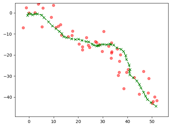
In the next plot (and throughout this section), the green crosses are the unobserved true path.
Show code cell source
plt.plot(x[0,:], x[1,:],
         marker='x', c='g', linestyle='dashed')
plt.xlim((np.min(x[0,:])-5, np.max(x[0,:])+5))
plt.ylim((np.min(x[1,:])-5, np.max(x[1,:])+5))
plt.scatter(y[0,:], y[1,:],
            c='r', alpha=0.5)
plt.show()
The following function implements the Kalman filter. The full recursion is broken up into several steps. We use numpy.linalg.inv to compute the Kalman gain matrix. Below, mu_pred is \(F \bmu_{t-1}\) and Sig_pred is \(P_{t-1} = F \bSigma_{t-1} F^T + Q\), which are the mean vector and covariance matrix of \(\bX_{t}\) given \(\bY_{1:t-1}\) as computed in the Predict step.
def kalmanUpdate(ss, F, H, Q, R, y_t, mu_prev, Sig_prev):
    mu_pred = F @ mu_prev
    Sig_pred = F @ Sig_prev @ F.T + Q
    e_t = y_t - H @ mu_pred
    S = H @ Sig_pred @ H.T + R
    Sinv = LA.inv(S)
    K = Sig_pred @ H.T @ Sinv
    mu_new = mu_pred + K @ e_t
    Sig_new = (np.diag(np.ones(ss)) - K @ H) @ Sig_pred
    return mu_new, Sig_new
def kalmanFilter(ss, os, y, F, H, Q, R, init_mu, init_Sig, T):
    mu = np.zeros((ss, T))
    Sig = np.zeros((ss, ss, T))
    mu[:,0] = init_mu
    Sig[:,:,0] = init_Sig

    for t in range(1,T):
        mu[:,t], Sig[:,:,t] = kalmanUpdate(ss, F, H, Q, R,
                                           y[:,t], mu[:,t-1],
                                           Sig[:,:,t-1])

    return mu, Sig
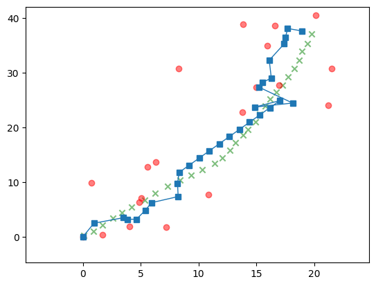
We apply this to the location tracking example. The inferred states, or more precisely their estimated mean, are in blue. Note that we also inferred the velocity at each time point, but we are not plotting that information.
init_mu = np.array([0., 0., 1., 1.])
init_Sig = 1 * np.diag(np.ones(ss))
mu, Sig = kalmanFilter(ss, os, y, F, H, Q, R, init_mu, init_Sig, T)
Show code cell source
plt.scatter(x[0,:], x[1,:],
            marker='x', c='g', alpha=0.5)
plt.xlim((np.min(x[0,:])-5, np.max(x[0,:])+5))
plt.ylim((np.min(x[1,:])-5, np.max(x[1,:])+5))
plt.scatter(y[0,:], y[1,:],
            c='r', alpha=0.5)
plt.plot(mu[0,:], mu[1,:],
         c='b', marker='s', linewidth=1)
plt.show()
To quantify the improvement in the inferred means compared to the observations, we compute the mean squared error in both cases.
dobs = x[0:1,:] - y[0:1,:]
mse_obs = np.sqrt(np.sum(dobs**2))
print(mse_obs)
22.891982252201856
dfilt = x[0:1,:] - mu[0:1,:]
mse_filt = np.sqrt(np.sum(dfilt**2))
print(mse_filt)
9.778610100463018
We indeed observe a substantial reduction.
Missing data We can also allow for the possibility that some observations are missing. Imagine for instance losing GPS signal while going through a tunnel. The recursions above are still valid, with the only modification that the Update equations involving \(\bY_t\) are dropped at those times \(t\) where there is no observation. In Numpy, we can use NaN to indicate the lack of observation. (Alternatively, one can use the numpy.ma module.)
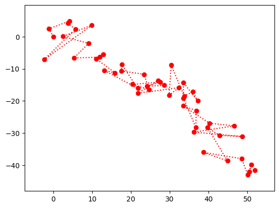
We use a same sample path as above, but mask observations at times \(t=10,\ldots,20\).
ss = 4
os = 2
F = np.array([[1., 0., 1., 0.],
              [0., 1., 0., 1.],
              [0., 0., 1., 0.],
              [0., 0., 0., 1.]])
H = np.array([[1., 0., 0., 0.],
              [0., 1, 0., 0.]])
Q = 0.01 * np.diag(np.ones(ss))
R = 10 * np.diag(np.ones(os))
init_mu = np.array([0., 0., 1., 1.])
init_Sig = Q
T = 30
x, y = lgSamplePath(ss, os, F, H, Q, R, init_mu, init_Sig, T)
for i in range(10,20):
    y[0,i] = np.nan
    y[1,i] = np.nan
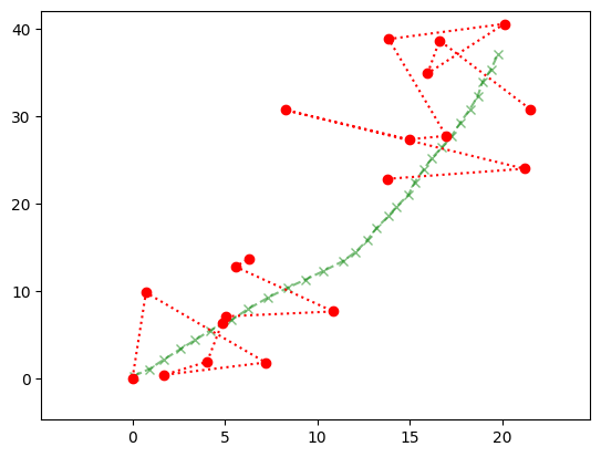
Here is the sample we are aiming to infer.
Show code cell source
plt.plot(x[0,:], x[1,:],
         marker='x', c='g', linestyle='dashed', alpha=0.5)
plt.xlim((np.min(x[0,:])-5, np.max(x[0,:])+5))
plt.ylim((np.min(x[1,:])-5, np.max(x[1,:])+5))
plt.plot(y[0,:], y[1,:],
         c='r', marker='o', linestyle='dotted')
plt.show()
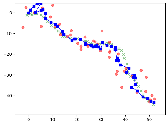
We modify the recursion accordingly, that is, skip the Update step when there is no observation to use for the update.
def kalmanUpdate(ss, F, H, Q, R, y_t, mu_prev, Sig_prev):
    mu_pred = F @ mu_prev
    Sig_pred = F @ Sig_prev @ F.T + Q
    if np.isnan(y_t[0]) or np.isnan(y_t[1]):
        return mu_pred, Sig_pred
    else:
        e_t = y_t - H @ mu_pred
        S = H @ Sig_pred @ H.T + R
        Sinv = LA.inv(S)
        K = Sig_pred @ H.T @ Sinv
        mu_new = mu_pred + K @ e_t
        Sig_new = (np.diag(np.ones(ss)) - K @ H) @ Sig_pred
        return mu_new, Sig_new
init_mu = np.array([0., 0., 1., 1.])
init_Sig = 1 * np.diag(np.ones(ss))
mu, Sig = kalmanFilter(ss, os, y, F, H, Q, R, init_mu, init_Sig, T)
Show code cell source
plt.scatter(x[0,:], x[1,:],
         marker='x', c='g', alpha=0.5)
plt.xlim((np.min(x[0,:])-5, np.max(x[0,:])+5))
plt.ylim((np.min(x[1,:])-5, np.max(x[1,:])+5))
plt.scatter(y[0,:], y[1,:],
            c='r', alpha=0.5)
plt.plot(mu[0,:], mu[1,:],
         marker='s', linewidth=1)
plt.show()