
\(\newcommand{\P}{\mathbb{P}}\) \(\newcommand{\E}{\mathbb{E}}\) \(\newcommand{\S}{\mathcal{S}}\) \(\newcommand{\X}{\mathcal{X}}\) \(\newcommand{\var}{\mathrm{Var}}\) \(\newcommand{\btheta}{\boldsymbol{\theta}}\) \(\newcommand{\bbeta}{\boldsymbol{\beta}}\) \(\newcommand{\bphi}{\boldsymbol{\phi}}\) \(\newcommand{\bpi}{\boldsymbol{\pi}}\) \(\newcommand{\bmu}{\boldsymbol{\mu}}\) \(\newcommand{\bSigma}{\boldsymbol{\Sigma}}\) \(\newcommand{\balpha}{\boldsymbol{\alpha}}\) \(\newcommand{\indep}{\perp\!\!\!\perp}\) \(\newcommand{\bLambda}{\boldsymbol{\Lambda}}\)
7.2. Background: introduction to parametric families and maximum likelihood estimation#
We introduce the basic building blocks in constructing probabilistic models. We introduce a common family of distributions, the exponential family.
Throughout this topic, all formal proofs are done under the assumption of a discrete distribution with finite support to avoid unnecessary technicalities and focus on the concepts. But everything we discuss can be adapted to continuous distributions.
Parametric families of probability distributions serve as basic building blocks for more complex models. By this, we mean a collection \(\{p_{\btheta}:\btheta \in \Theta\}\), where \(p_{\btheta}\) is a probability distribution over a set \(\S_{\btheta}\) and \(\btheta\) is a vector-valued parameter.
EXAMPLE: (Bernoulli) The random variable \(X\) is Bernoulli with parameter \(q \in [0,1]\), denoted \(X \sim \mathrm{Ber}(q)\), if it takes values in \(\S_X = \{0,1\}\) and \(\P[X=1] = q\). Varying \(q\) produces the family of Bernoulli distributions. \(\lhd\)
Here we focus on exponential families, which include many common distributions (including the Bernoulli distribution).
7.2.1. Exponential family#
One particularly useful class of probability distributions in data science is the exponential family, which includes many well-known cases.
DEFINITION (Exponential Family - Discrete Case) A parametric collection of probability distributions \(\{p_{\btheta}:\btheta \in \Theta\}\) over a discrete space \(\S\) is an exponential family if it can be written in the form
where \(\btheta \in \mathbb{R}^m\) are the canonical parameters, \(\bphi : \S \to \mathbb{R}^m\) are the sufficient statistics and \(Z(\btheta)\) is the partition function. It is often convenient to introduce the function \(A(\btheta) = \log Z(\btheta)\) and re-write
\(\natural\)
EXAMPLE: (Bernoulli, continued) For \(x \in \{0,1\}\), the \(\mathrm{Ber}(q)\) distribution for \(0 < q < 1\) can be written as
where we define \(h(x) = 1\), \(\phi(x) = x\), \(\theta = \log \left(\frac{q}{1-q}\right)\) and, since \(Z(\theta)\) serves as the normalization constant in \(p_\theta\),
\(\lhd\)
The following is an important generalization.
EXAMPLE: (Categorical and Multinomial) A categorical variable \(X\) takes \(K \geq 2\) possible values. A standard choice is to use one-hot encoding \(\S = \{\mathbf{e}_i : i=1,\ldots,K\}\) where \(\mathbf{e}_i\) is the \(i\)-th canonical basis in \(\mathbb{R}^K\). The distribution is specified by setting the probabilities \(\bpi = (\pi_1,\ldots,\pi_K)\)
We denote this \(X \sim \mathrm{Cat}(\bpi)\) and we assume \(\pi_i > 0\) for all \(i\).
To see that this is an exponential family, write the probability mass function at \(\mathbf{x} = (x_1,\ldots,x_K)\) as
So we can take \(h(\mathbf{x}) = 1\), \(\btheta = (\log \pi_i)_{i=1}^K\), \(\bphi(\mathbf{x}) = (x_i)_{i=1}^K\) and \(Z(\btheta) = 1\).
The multinomial distribution arises as a sum of independent categorical variables. Let \(n \geq 1\) be the number of trials (or samples) and let \(Y_1,\ldots,Y_n\) be i.i.d. \(\mathrm{Cat}(\bpi)\). Define \(X = \sum_{i=1}^n Y_i\). The probability mass function of \(X\) at
is
and we can take \(h(\mathbf{x}) = \frac{n!}{x_1!\cdots x_K!}\), \(\btheta = (\log \pi_i)_{i=1}^K\), \(\bphi(\mathbf{x}) = (x_i)_{i=1}^K\) and \(Z(\btheta) = 1\). This is an exponential family if we think of \(n\) as fixed.
We use the notation \(X \sim \mathrm{Mult}(n, \bpi)\). \(\lhd\)
While we have focused so far on discrete distributions, one can adapt the definitions above by replacing mass functions with density functions. We give two important examples.
We need some definitions for our first example.
The trace of a square matrix \(A \in \mathbb{R}^{d \times d}\), denoted \(\mathrm{tr}(A)\), is the sum of its diagonal entries. We will need the following trace identity whose proof we leave as an exercise: \(\mathrm{tr}(ABC) = \mathrm{tr}(CAB) = \mathrm{tr}(BCA)\) for any matrices \(A, B, C\) for which \(AB\), \(BC\) and \(CA\) are well-defined.
The determinant of a square matrix \(A\) is denoted by \(|A|\). For our purposes, it will be enough to consider symmetric, positive semidefinite matrices for which the determinant is the product of the eigenvalues. Recall that we proved that the sequence of eigenvalues (with repeats) of a symmetric matrix is unique (in the sense that any two spectral decomposition have the same sequence of eigenvalues).
A symmetric, positive definite matrix \(A \in \mathbb{R}^{d \times d}\) is necessarily invertible. Indeed, it has a spectral decomposition
where \(\lambda_1 \geq \cdots \geq \lambda_d > 0\) and \(\mathbf{q}_1, \ldots, \mathbf{q}_d\) are orthonormal. Then
To see this, note that
The last equality follows from the fact that \(Q Q^T\) is the orthogonal projection on the orthonormal basis \(\mathbf{q}_1,\ldots,\mathbf{q}_d\). Similarly, \(A^{-1} A = I_{d \times d}\).
EXAMPLE: (Multivariate Gaussian) A multivariate Gaussian vector \(\mathbf{X} = (X_1,\ldots,X_d)\) on \(\mathbb{R}^d\) with mean \(\bmu \in \mathbb{R}^d\) and positive definite covariance matrix \(\bSigma \in \mathbb{R}^{d \times d}\) has probability density function
We use the notation \(\mathbf{X} \sim N_d(\bmu, \bSigma)\).
It can be shown that indeed the mean is
and the covariance matrix is
See, e.g., [Bis, Secion 2.3].
In the bivariate case (i.e., when \(d = 2\)), the covariance matrix reduces to
where \(\sigma_1^2\) and \(\sigma_2^2\) are the respective variances of \(X_1\) and \(X_2\), and
is the correlation coefficient. Recall that, by Cauchy-Schwarz, it lies in \([-1,1]\).
The following code, which plots the density in the bivariate case, was adapted from gauss_plot_2d.ipynb by ChatGPT.
LEARNING BY CHATTING: Ask your favorite AI chatbot to explain the code! Try different covariance matrices. \(\ddagger\)
from scipy.stats import multivariate_normal

def gaussian_pdf(X, Y, mean, cov):
    xy = np.stack([X.flatten(), Y.flatten()], axis=-1)
    return multivariate_normal.pdf(
        xy, mean=mean, cov=cov).reshape(X.shape)
Show code cell source
def make_surface_plot(X, Y, Z):
    fig = plt.figure()
    ax = fig.add_subplot(111, projection='3d')
    surf = ax.plot_surface(
        X, Y, Z, cmap=plt.cm.viridis, antialiased=False)
    plt.show()
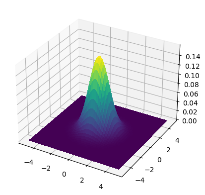
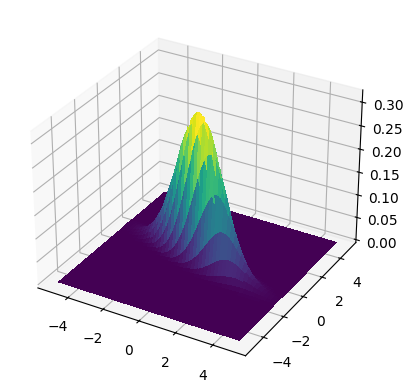
We plot the density for mean \((0,0)\) with two different covariance matrices:
where \(\sigma_1 = 1.5\), \(\sigma_2 = 0.5\) and \(\rho = -0.75\).
Show code cell source
start_point = 5
stop_point = 5
num_samples = 100
points = np.linspace(-start_point, stop_point, num_samples)
X, Y = np.meshgrid(points, points)

mean = np.array([0., 0.])
cov = np.array([[1., 0.], [0., 1.]])
make_surface_plot(X, Y, gaussian_pdf(X, Y, mean, cov))
Show code cell source
mean = np.array([0., 0.])
cov = np.array([[1.5 ** 2., -0.75 * 1.5 * 0.5],
                 [-0.75 * 1.5 * 0.5, 0.5 ** 2.]])
make_surface_plot(X, Y, gaussian_pdf(X, Y, mean, cov))
Rewriting the density as
where we used the symmetric nature of \(\bSigma^{-1}\) in the first term of the exponential and the previous trace identity in the second term. The expression in parentheses is linear in the entries of \(\mathbf{x}\) and \(\mathbf{x} \mathbf{x}^T\), which can then be taken as sufficient statistics (formally, using vectorization). Indeed note that
and
So we can take
and \(h (\mathbf{x}) \equiv 1\). Expressing \(Z(\btheta)\) explicitly is not straightforward. But note that \(\btheta\) includes all entries of \(\bSigma^{-1}\), from which \(\bSigma\) can be computed (e.g., from Cramer’s rule), and in turn from which \(\bmu\) can be extracted out of the entries of \(\bSigma^{-1}\bmu\) in \(\btheta\). So the normalizing factor \(\frac{(2\pi)^{d/2} \,|\bSigma|^{1/2}}{e^{-(1/2) \bmu^T \bSigma^{-1} \bmu}}\) can in principle be expressed in terms of \(\btheta\).
This shows that the multivariate normal is an exponential family.
The matrix \(\bLambda = \bSigma^{-1}\) is also known as the precision matrix.
Alternatively, let \(\mathbf{Z}\) be a standard Normal \(d\)-vector, let \(\bmu \in \mathbb{R}^d\) and let \(\bSigma \in \mathbb{R}^{d \times d}\) be positive definite. Then the transformed random variable \(\mathbf{X} = \bmu + \bSigma \mathbf{Z}\) is a multivariate Gaussian with mean \(\bmu\) and covariance matrix \(\bSigma\). This can be proved using the change of variables formula (try it!). \(\lhd\)
The Dirichlet distribution, which we describe next, is a natural probability distribution over probability distributions. In particular, it is used in Bayesian data analysis as a prior on the parameters of categorical and multinomial distribution, largely because of a property known as conjuguacy. We will not describe Bayesian approaches here.
EXAMPLE: (Dirichlet) The Dirichlet distribution is a distribution over the \((K-1)\)-simplex
Its parameters are \(\balpha = (\alpha_1, \ldots, \alpha_K) \in \mathbb{R}\) and the density is
where the normalizing constant \(B(\balpha)\) is the multivariate Beta function.
Rewriting the density as
shows that this is an exponential family with the canonical parameters \(\balpha\) and sufficient statistics \((\log x_i)_{i=1}^K\). \(\lhd\)
See here for many more examples. Observe, in particular, that the same distribution can have several representations as an exponential family.
NUMERICAL CORNER: In Numpy, as we have seen before, the module numpy.random provides a way to sample from a variety of standard distributions. We first initialize the pseudorandom number generator with a random seed. Recall that it allows the results to be reproducible: using the same seed produces the same results again.
seed = 535
rng = np.random.default_rng(535)
Here’s are lists of available probability distributions.
p = 0.1 # probability of success
N = 5 # number of samples
rng.binomial(1, p, size=N) # Bernoulli is special case of binomial with 1 trial
array([1, 0, 0, 0, 0])
Here are a few other examples.
p = [0.1, 0.2, 0.7]
n = 100
rng.multinomial(n, p, size=N)
array([[ 9, 12, 79],
       [ 5, 20, 75],
       [13, 18, 69],
       [ 8, 18, 74],
       [ 8, 24, 68]])
mu = np.array([0.1, -0.3])
sig = np.array([[2., 0.],[0., 3.]])
rng.multivariate_normal(mu, sig, size=N)
array([[-0.7275232 ,  2.66555155],
       [ 0.45641186, -2.65834344],
       [ 1.13188325,  0.43920735],
       [ 0.69846716,  2.49891659],
       [ 0.91725117,  1.89618733]])
\(\unlhd\)
MULTIPLE CHOICE: The Weibull distribution with known shape parameter \(k > 0\) takes the following form
for \(x \geq 0\), where \(\lambda > 0\).
What is the sufficient statistic of its exponential family form?
a) \(x\)
b) \(\log x\)
c) \(x^{k-1}\)
d) \(x^k\)
e) \((\log x, x^k)\)
\(\ddagger\)
7.2.2. Parameter estimation#
When modeling data via a parametric family of distributions, the parameters must be determined from the data itself. In a typical setting, we assume that the data comprises \(n\) independent samples \(\mathbf{X}_1,\ldots,\mathbf{X}_n\) from a parametric family \(p_{\btheta}\) with unknown \(\btheta \in \Theta\). Many methods exist for estimating \(\btheta\), depending on the context. Here we focus on maximum likelihood estimation. It has many good theoretical properties which we will not describe here, as well as drawbacks.
The idea behind maximum likelihood estimation is simple and intuitive: we choose the parameter that maximizes the probability of observing the data.
DEFINITION (Maximum likelihood estimator) Assume that \(\mathbf{X}_1,\ldots,\mathbf{X}_n\) are \(n\) independent samples from a parametric family \(p_{\btheta^*}\) with unknown \(\btheta^* \in \Theta\). The maximum likelihood estimator of \(\btheta\) is defined as
It is often useful to work with the negative log-likelihood (NLL)
in which case we are miniziming. \(\natural\)
EXAMPLE: (Biased coin) Suppose we observe \(n\) coin flips \(X_1,\ldots, X_n \in \{0,1\}\) from a biased coin with an unknown probability \(\theta^*\) of producing \(1\). We assume the flips are independent. We compute the MLE of the parameter \(\theta\).
The definition is
where, using our previous Bernoulli example, the NLL is
We compute the first and second derivatives of \(L_n(\theta; \{X_i\}_{i=1}^n)\) as a function of \(\theta\):
and
The second derivative is non-negative and therefore the NLL is convex. To find a global minimizer, it suffices to find a stationary point.
We make the derivative of the NLL equal to \(0\)
So
This is in fact a natural estimator: the empirical frequency of \(1\)s. \(\lhd\)
We give an alternative perspective on the maximum likelihood estimator. Assume that \(p_{\btheta}\) is supported on a fixed finite set \(\X\) for all \(\btheta \in \Theta\). Given samples \(\mathbf{X}_1,\ldots,\mathbf{X}_n\), for each \(\mathbf{x} \in \X\), let
count the number of times \(\mathbf{x}\) is observed in the data and let
be the empirical frequency of \(\mathbf{x}\) in the sample. Observe that \(\hat\mu_n\) is a probability distribution over \(\X\).
The following theorem characterizes the maximum likelihood estimator in terms of the Kullback-Liebler divergence, which was introduced in a previous section.
For two probability distributions
it is defined as
where it will suffice to restrict ourselves to the case \(\mathbf{q} > \mathbf{0}\) and where we use the convention \(0 \log 0 = 0\) (so that terms with \(p_i = 0\) contribute \(0\) to the sum).
Notice that \(\mathbf{p} = \mathbf{q}\) implies \(\mathrm{KL}(\mathbf{p} \| \mathbf{q}) = 0\). We show that \(\mathrm{KL}(\mathbf{p} \| \mathbf{q}) \geq 0\), a result known as Gibbs’ inequality. (A quick look at the proof shows that the result holds as long as \(\sum_{i=1}^K q_i \leq 1\) instead of \(\sum_{i=1}^K q_i = 1\). )
THEOREM (Gibbs) For any \(\mathbf{p}, \mathbf{q} \in \Delta_K\) with \(\mathbf{q} > \mathbf{0}\),
\(\sharp\)
Proof: Let \(I\) be the set of indices \(i\) such that \(p_i > 0\). Hence
It can be proved that \(\log x \leq x - 1\) for all \(x > 0\) (Try it!). So
where we used that \(\log z^{-1} = - \log z\) on the first line and the fact that \(p_i = 0\) for all \(i \notin I\) on the fourth line. \(\square\)
THEOREM (MLE via KL) Assume that, for all \(\btheta \in \Theta\), \(p_{\btheta}\) is supported on a fixed finite set \(\X\) and that \(p_{\btheta}(\mathbf{x}) > 0\) for all \(\mathbf{x} \in \X\). Given samples \(\mathbf{X}_1,\ldots,\mathbf{X}_n\) from \(p_{\btheta^*}\), let \(\{\hat\mu_n(\mathbf{x})\}_{\mathbf{x} \in \X}\) be the corresponding empirical frequencies. Then the maximum likelihood estimator \(\hat\btheta_{\mathrm{MLE}}\) of \(\btheta\) is also a solution to
\(\sharp\)
Proof idea: Manipulate the negative log-likelihood to bring out its relationship to the Kullback-Liebler divergence.
Proof: We can re-write the negative log-likelihood as
To bring out the Kullback-Liebler divergence, we further transform the previous equation into
where the second term is referred to as the entropy of \(\hat\mu_n\).
Because \(\mathrm{H}(\hat\mu_n)\) does not depend on \(\btheta\), minimizing \(L_n(\btheta; \{\mathbf{X}_i\}_{i=1}^n)\) is equivalent to minimizing \(\mathrm{KL}(\hat{\mu}_n \| p_{\btheta})\) as claimed. \(\square\)
In words, the maximum likelihood estimator chooses the parametric distribution that is closest to \(\hat\mu_n\) in Kullback-Liebler divergence. One can think of this as projecting \(\hat\mu_n\) onto the space \(\{p_{\btheta} : \btheta \in \Theta\}\) under the Kullback-Liebler notion of distance.
EXAMPLE: (Special case) One special case is where \(\X\) is finite, \(\btheta = (\theta_\mathbf{x})_{\mathbf{x} \in \X}\) is a probability distribution over \(\X\), and \(p_{\btheta} = \btheta\). That is, we consider the class of all probability distributions over \(\X\). Given samples \(\mathbf{X}_1,\ldots,\mathbf{X}_n\) from \(p_{\btheta^*}\), in this case we have
where recall that, by convention, if \(\hat\mu_n(\mathbf{x}) = 0\) then \(\hat\mu_n(\mathbf{x}) \log \frac{\hat\mu_n(\mathbf{x})}{\theta_\mathbf{x}} = 0\) for any \(\theta_\mathbf{x}\). So, letting \(\mathbb{X}_n = \{\mathbf{X}_1,\ldots,\mathbf{X}_n\}\) be the set of distinct values encountered in the sample (ignoring repetitions), we have
Note that \(\sum_{\mathbf{x} \in \mathbb{X}_n} \hat\mu_n(\mathbf{x}) = 1\).
We have previously established Gibbs’ inequality which says that: for any \(\mathbf{p}, \mathbf{q} \in \Delta_K\) with \(\mathbf{q} > \mathbf{0}\), it holds that \(\mathrm{KL}(\mathbf{p} \| \mathbf{q}) \geq 0\).
The minimum \(\mathrm{KL}(\hat{\mu}_n \| p_{\btheta}) = 0\) can be achieved by setting \(\btheta_{\mathbf{x}} = \hat\mu_n(\mathbf{x})\) for all \(\mathbf{x} \in \mathbb{X}_n\) and \(\btheta_{\mathbf{x}} = 0\) for all \(\mathbf{x} \notin \mathbb{X}_n\). The condition
is then satisfied.
So in this case \(\hat\mu_n\) is a maximum likelihood estimator.
A special case of this is the biased coin example. \(\lhd\)
7.2.3. Parameter estimation for exponential families#
For exponential families, maximum likelihood estimation takes a particularly natural form. We provide details in the discrete case.
THEOREM (Maximum Likelihood Estimator for Exponential Families) Assume that \(p_{\btheta}\) takes the exponential family form
that the support \(\S\) is finite, and that \(A\) is twice continuously differentiable over the open set \(\Theta\). Let \(\mathbf{X}_1,\ldots,\mathbf{X}_n\) be \(n\) independent samples from a parametric family \(p_{\btheta^*}\) with unknown \(\btheta^* \in \Theta\). Then \(L_n(\btheta; \{\mathbf{X}_i\}_{i=1}^n)\), as a function of \(\btheta\), is convex and the maximum likelihood estimator of \(\btheta\) – if it exists – solves the system of moment-matching equations
where \(\mathbf{X} \sim p_{\hat\btheta_{\mathrm{MLE}}}\). \(\sharp\)
We will need some auxiliary formulas and results. Recall the following definition:
DEFINITION (Covariance matrix) Let \(\mathbf{Z}\) be a random vector. The covariance matrix of \(\mathbf{Z}\) is defined as
\(\natural\)
It is also sometimes denoted as \(\bSigma_\mathbf{Z}\).
We give a second proof of the following result, encountered previously.
LEMMA Let \(\mathbf{Z}\) be a random vector taking values in \(\mathbb{R}^m\) whose components have finite variances. Then the covariance matrix of \(\mathbf{Z}\), \(\mathrm{K}_{\mathbf{Z}, \mathbf{Z}}\), is positive semidefinite. \(\flat\)
Proof idea: We show that the quadratic form \(\langle \mathbf{y}, \mathrm{K}_{\mathbf{Z}, \mathbf{Z}} \mathbf{y}\rangle\) can be written as a variance, and so is always non-negative.
Proof: For any \(\mathbf{y} \in \mathbb{R}^m\), by the exercise above,
Since this inequality holds for any \(\mathbf{y}\), it follows by definition that \(\mathrm{K}_{\mathbf{Z}, \mathbf{Z}} \succeq 0\). \(\square\)
The function \(A\) has properties worth highlighting that will be used in the proof.
LEMMA (Derivatives of \(A\)) Assume that \(p_{\btheta}\) takes the exponential family form
that the support \(\S\) is finite, and that \(A\) is twice continuously differentiable over the open set \(\Theta\). Then
where \(\mathbf{X} \sim p_{\btheta}\). \(\flat\)
Proof idea: Follows from a direct calculation.
Proof: We observe first that
where we used the fact that, by definition, \(Z(\btheta)\) is the normalization constant of \(p_{\btheta}\). In particular, as the logarithm of a finite, weighted sum of exponentials, the function \(A(\btheta)\) is continuously differentiable. Hence so is \(p_{\btheta}(\mathbf{x})\) as a function of \(\btheta\).
From the formula above and the basic rules of calculus,
where \(\mathbf{X} \sim p_{\btheta}\).
Differentiating again, this time with respect to \(\theta_i\), we obtain
where again \(\mathbf{X} \sim p_{\btheta}\). That concludes the proof. \(\square\)
We are now ready to the prove the main theorem.
Proof: (Maximum Likelihood Estimator for Exponential Families) We begin by computing the stationary points of the log-likelihood, for which we need the gradient with respect to \(\btheta \in \mathbb{R}^m\). We will also need the second-order derivatives to establish convexity. We have
and
We use the expressions for the derivatives of \(A\) obtained above.
Plugging into the formula for the minus log-likelihood (as a function of \(\btheta\)), we get for the gradient with respect to \(\btheta\)
This is also known in statistics as the score.
For the Hessian with respect to \(\btheta\), we get
This is also known in statistics as the observed information. (In fact, in this case, it reduces to the Fisher information.) Since \(\mathrm{K}_{\bphi(\mathbf{X}), \bphi(\mathbf{X})}\) is positive semidefinite, so is \(\mathbf{H}_{L_n}(\btheta; \{\mathbf{X}_i\}_{i=1}^n)\).
Hence, a stationary point \(\hat\btheta_{\mathrm{MLE}}\) must satisfy
where \(\mathbf{X} \sim p_{\hat\btheta_{\mathrm{MLE}}}\) or, after re-arranging,
Because \(L_n\) is convex, a stationary point – if it exists – is necessarily a global minimum (and vice versa) by the First-Order Sufficient Condition for Convex Functions. \(\square\)
EXAMPLE: (Bernoulli/biased coin, continued) For \(x \in \{0,1\}\), recall that the \(\mathrm{Ber}(q)\) distribution can be written as
where we define \(h(x) = 1\), \(\phi(x) = x\), \(\theta = \log \left(\frac{q}{1-q}\right)\) and \(Z(\theta) = \sigma(\theta)\). Let \(X_1,\ldots,X_n\) be independent samples from \(p_{\theta^*}\).
For \(X \sim p_{\hat\theta_{\mathrm{MLE}}}\), the moment-matching equations reduce to
To compute the left-hand side in terms of \(\hat\theta_{\mathrm{MLE}}\) we use the relationship \(\theta = \log \left(\frac{q}{1-q}\right)\), that is,
Hence, \(\hat\theta_{\mathrm{MLE}}\) is well-defined when \(\frac{1}{n} \sum_{i=1}^n X_i \neq 0, 1\).
Define \(q^*\) as the solution to
that is,
where \(\sigma\) is the sigmoid function.
By the law of large numbers, as \(n \to +\infty\), we get the convergence
with probability one.
Because the function \(\log \left(\frac{q}{1-q}\right)\) is continuous for \(q \in (0,1)\), we have furthermore
In words, the maximum likelihood estimator \(\hat\theta_{\mathrm{MLE}}\) is guaranteed to converge to the true parameter \(\theta^*\) when the number of samples grows. This fundamental property is known as statistical consistency. \(\lhd\)
Statistical consistency holds more generally for the maximum likelihood estimator under exponential families (and parametric families more broadly), provided certain technical conditions hold. We will not provide further details here.
Unlike the previous example, one does not always have an explicit formula for the maximum likelihood estimator under exponential families. Instead, optimization methods, for instance Newton’s method described in a previous assignment, are used in such cases.
EXAMPLE: (Multivariate Gaussian) We established the theorem for finite \(\mathcal{S}\), but it holds more generally. Consider the multivariate Gaussian case. Here the sufficient statistics are
which is simply the vector \(\mathbf{x}\) itself stacked with the vectorized form of the matrix \(\mathbf{x} \mathbf{x}^T\). So the moment-matching equations boil down to
and
The first equation says to choose \(\bmu = \frac{1}{n} \sum_{i=1}^n \mathbf{X}_i\). The second one says to take
\(\lhd\)
THINK-PAIR-SHARE: Consider again the Weibull distribution with known shape parameter \(k > 0\).
a) Compute \(\E[X^k]\). [Hint: Perform a change of variables.]
b) What is the MLE of \(\lambda\)?
\(\ddagger\)
7.2.4. Generalized linear models#
Generalized linear models provide a vast generalization of linear regression using exponential families. Quoting from Wikipedia, the context in which they arise is the following:
Ordinary linear regression predicts the expected value of a given unknown quantity (the response variable, a random variable) as a linear combination of a set of observed values (predictors). This implies that a constant change in a predictor leads to a constant change in the response variable (i.e. a linear-response model). This is appropriate when the response variable can vary, to a good approximation, indefinitely in either direction, or more generally for any quantity that only varies by a relatively small amount compared to the variation in the predictive variables, e.g. human heights. However, these assumptions are inappropriate for some types of response variables.
For example, in cases where the response variable is expected to be always positive and varying over a wide range, constant input changes lead to geometrically (i.e. exponentially) varying, rather than constantly varying, output changes. […] Similarly, a model that predicts a probability of making a yes/no choice (a Bernoulli variable) is even less suitable as a linear-response model, since probabilities are bounded on both ends (they must be between 0 and 1). […] Generalized linear models cover all these situations by allowing for response variables that have arbitrary distributions (rather than simply normal distributions), and for an arbitrary function of the response variable (the link function) to vary linearly with the predicted values (rather than assuming that the response itself must vary linearly).
In its simplest form, a generalized linear model assumes that an outcome variable \(y \in \mathbb{R}\) is generated from an exponential family \(p_\theta\), where \(\theta \in \mathbb{R}\) is a linear combination of the predictor variables \(\mathbf{x} \in \mathbb{R}^d\). That is, we assume that \(\theta = \mathbf{w}^T \mathbf{x}\) for unknown \(\mathbf{w} \in \mathbb{R}^d\) and the probability distribution of \(y\) is of the form
for some sufficient statistic \(\phi(y)\). We further assume that \(A\) is twice continuously differentiable over \(\mathbb{R}\).
Given data points \((\mathbf{x}_i,y_i)_{i=1}^n\), the model is fitted using maximum likelihood as follows. Under independence of the samples, the likelihood of the data is \(\prod_{i=1}^n p_{\mathbf{w}^T \mathbf{x}_i}(y_i)\), which we seek to maximize over \(\mathbf{w}\) (which is different from maximizing over \(\theta\)!). As before, we work with the negative log-likelihood, which we denote as (with a slight abuse of notation)
The gradient with respect to \(\mathbf{w}\) is given by
By the Chain Rule and our previous formulas,
where \(\mu(\mathbf{w}; \mathbf{x}_i) = \E[\phi(Y_i)]\) with \(Y_i \sim p_{\mathbf{w}^T \mathbf{x}_i}\). That is,
The Hessian of \(A(\mathbf{w}^T \mathbf{x}_i)\), again by the Chain Rule and our previous formulas, is
where \(\sigma^2(\mathbf{w}; \mathbf{x}_i) = \mathrm{K}_{\phi(Y_i), \phi(Y_i)} = \var[\phi(Y_i)]\) with \(Y_i \sim p_{\mathbf{w}^T \mathbf{x}_i}\). So the Hessian of the negative log-likelihood is
which is positive semidefinite (prove it!).
As a result, the negative log-likelihood is convex and the maximum likelihood estimator \(\hat{\mathbf{w}}_{\mathrm{MLE}}\) solves the equation \(\nabla_\mathbf{w} L_n(\mathbf{w};\{(\mathbf{x}_i,y_i)_{i=1}^n\}) = \mathbf{0}\), that is,
We revisit linear and logistic regression next.
EXAMPLE: (Linear regression) Consider the case where \(p_\theta\) is a univariate Gaussian with mean \(\theta\) and fixed variance \(1\). That is,
where \(\phi(y) = y\) and \(A(\theta) = \theta^2/2\). We now assume that \(\theta = \mathbf{x}^T \mathbf{w}\) to obtain the corresponding generalized linear model.
Given data points \((\mathbf{x}_i,y_i)_{i=1}^n\), recall that the maximum likelihood estimator \(\hat{\mathbf{w}}_{\mathrm{MLE}}\) solves the equation
where \(\mu(\mathbf{w}; \mathbf{x}_i) = \E[\phi(Y_i)]\) with \(Y_i \sim p_{\mathbf{x}_i^T \mathbf{w}}\). Here \(\E[\phi(Y_i)] = \E[Y_i] = \mathbf{x}_i^T \mathbf{w}\). So the equation reduces to
You may not recognize this equation, but we have encountered it before in a different form. Let \(A\) be the matrix with row \(i\) equal to \(\mathbf{x}_i\) and let \(\mathbf{y}\) be the vector with \(i\)-th entry equal to \(y_i\). Then
as can be checked entry by entry or by using our previous characterizations of matrix-matrix products (in outer-product form) and matrix-vector products (as linear combinations of columns). Therefore, the equation above is equivalent to \(A^T A \mathbf{w} = A^T \mathbf{y}\) - the normal equations of linear regression.
To make sense of this finding, we look back at the minus log-likelihood
Observe that mimizing this expression over \(\mathbf{w}\) is equivalent to solving the least-squares problem as the first term does not depend on \(\mathbf{w}\) and the factor of \(1/2\) does not affect the optimum.
While we have rederived the least squares problem from a probabilistic model, it should be noted that the Gaussian assumption is not in fact required for linear regression to be warranted. Rather, it gives a different perspective on the same problem. \(\lhd\)
EXAMPLE: (Logistic regression) Consider the case where \(p_{\theta}\) is a Bernoulli distribution. That is, for \(y \in \{0,1\}\),
where \(h(y) = 1\), \(\phi(y) = y\) and \(A(\theta) = \log(1 + e^\theta)\). We assume that \(\theta = \mathbf{x}^T \mathbf{w}\) to obtain the corresponding generalized linear model. Given data points \((\mathbf{x}_i,y_i)_{i=1}^n\), the maximum likelihood estimator \(\hat{\mathbf{w}}_{\mathrm{MLE}}\) solves the equation
where \(\mu(\mathbf{w}; \mathbf{x}_i) = \E[\phi(Y_i)]\) with \(Y_i \sim p_{\mathbf{x}_i^T \mathbf{w}}\). Here, by our formula for the gradient of \(A\),
where \(\sigma\) is the sigmoid function. So the equation reduces to
The equation in this case cannot be solved explicitly. Instead we can use gradient descent, or a variant, to minimize the minus log-likelihood directly. The lattter is
Minimizing \(L_n(\mathbf{w};\{(\mathbf{x}_i,y_i)_{i=1}^n\})\) is equivalent to logistic regression.
To use gradient descent, we compute
This expression is indeed consistent with what we previously derived for logistic regression. \(\lhd\)
In practice, generalized linear models of moderate dimension are often fitted using the second-order method Iterative Reweighted Least Squares (IRLS), which generalizes the special case for logistic regression.